
Wormhole Culverts Part 2
Wormhole Island: Using a wormhole culvert to introduce internal boundary conditions into HEC-RAS 2D models
- Wormhole Culverts Part 1: Introducing the wormhole concept
- Wormhole Culverts Part 2: Using wormhole culverts for internal boundary conditions
- Wormhole Culverts Part 3: Comparing wormhole culverts to 1D/2D bridges and culverts
- Wormhole Culverts Part 4: Sensitivity analyses for wormhole culverts
- Wormhole Culverts Part 5: What’s the best shape for a wormhole culvert?
May 2018 update
[PLEASE NOTE: Wormhole culverts have become obsolete with the release of HEC-RAS Version 5.0.4. See our new article on what’s new in 5.0.4 for instructions and videos on using the new culvert options.]
In the current version of HEC-RAS, inflows can only be introduced along the external 2D Area boundary, and I frequently run up against this limitation. When a tributary’s headwaters are located completely within the 2D area, for example, I’ve had to use the “Pac-man Method” (putting a slice into my external boundary) just to introduce the inflow. This becomes problematic when there is flow on both sides of the inflow, however. By introducing an artificial upstream storage area outside of my area of interest (but inside of the 2D Area) and connecting it to my desired inflow location with a wormhole culvert, however, I can add inflows anywhere I’d like.
Wormhole culverts then essentially become a workaround for allowing internal boundary condition lines. Keep in mind, though, that the 500-point limitation on weir embankments still holds, and the weir elevations cannot be set below the ground level. The cross section points filter can be used to reduce the number of points for a long connection, but then some of the weir elevations will also need to be raised, so the process gets very awkward if you move the inflow and outflow locations too far apart.
Although the Wormhole Method is a bit cumbersome for this purpose (because it requires some trial and error to adjust the culvert outflow hydrograph to match the desired inflow hydrograph at the internal boundary condition location), it can be used in a pinch.
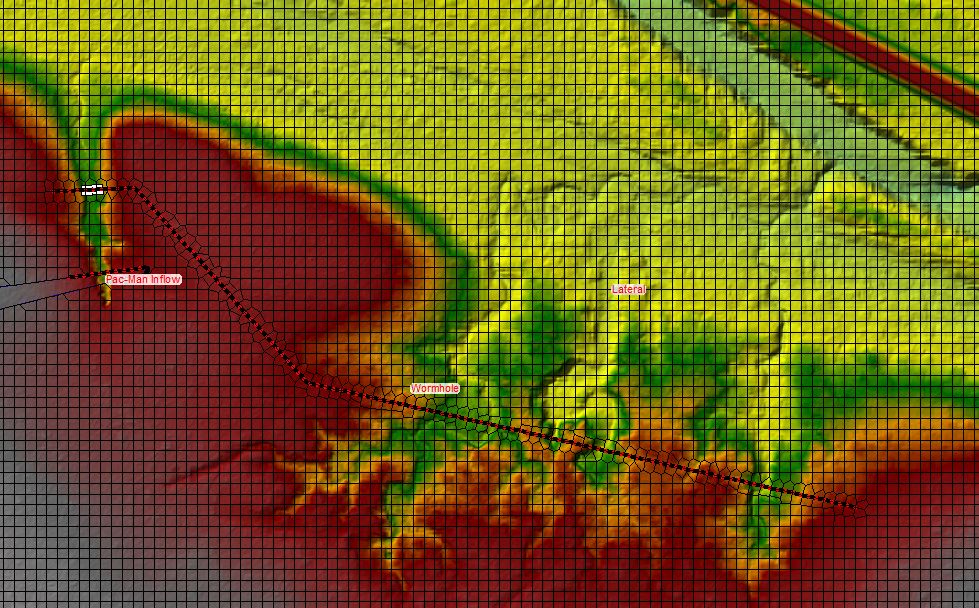
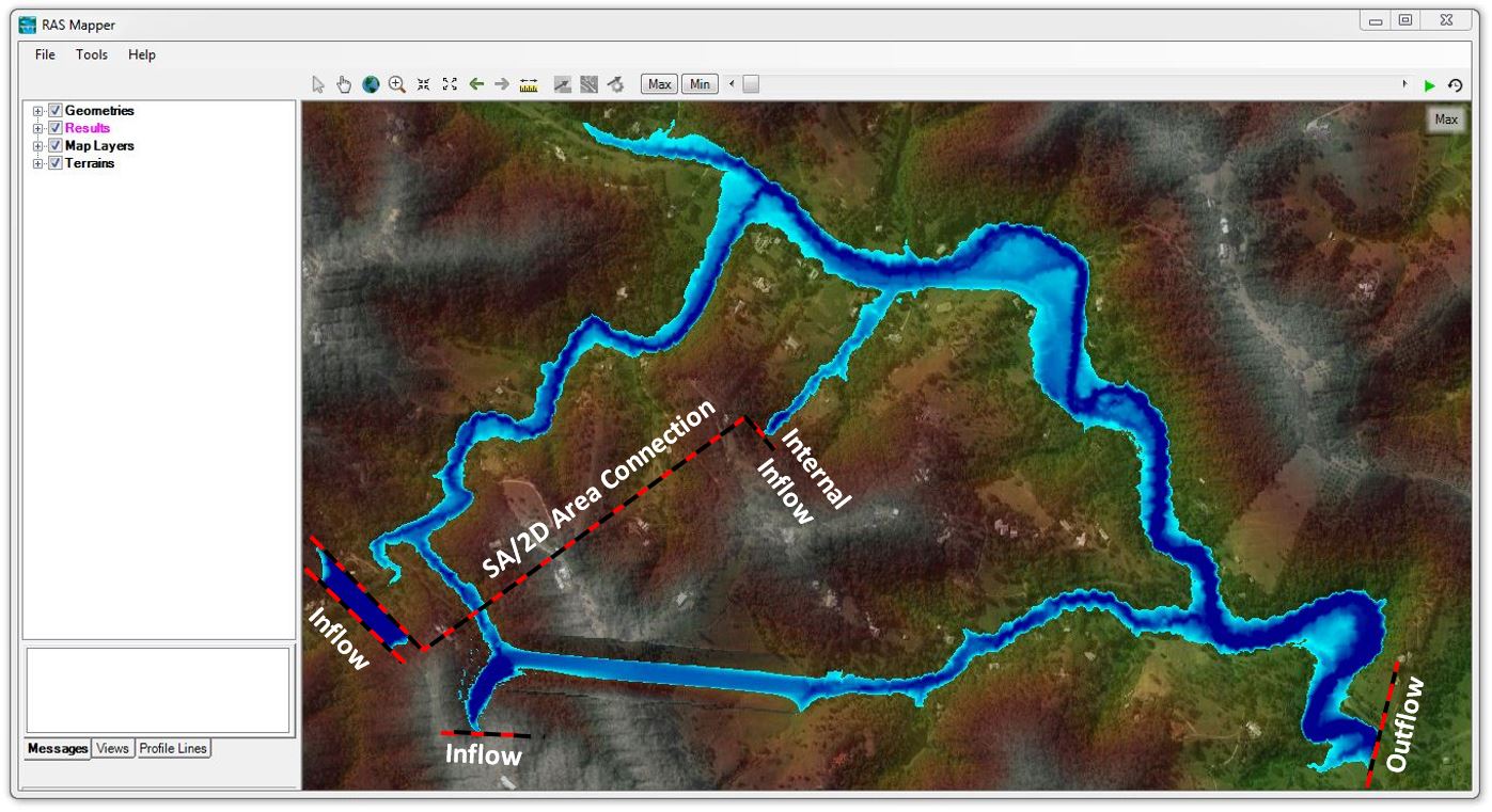
Below is an example that shows how to use a wormhole culvert (essentially a SA/2D Area Connection with upstream and downstream culvert centerline stations located some distance apart) to introduce an internal boundary condition. In the schematic below, I’ve assumed the tributary on the left is outside of my area of interest and that I want to bring some flow into the tributary on the right without moving the external boundary around that tributary. You can see what I mean by the “Pac-Man” method here (in case that designation isn’t as self-explanatory as I might think as a retro fan).
[I could just as well choose any area along the existing external boundary that doesn’t affect the hydraulic conditions in my area of interest.]
I then add an SA/2D Area Connection that crosses each of the tributaries as shown here:
I then edit the SA/2D Area Connection and click on the Weir/Embankment editor and copy/paste the terrain profile data into the weir/embankment profile. I add a culvert with the upstream station in the left channel and the downstream station in the right channel. Because there is no other flow crossing the connection line, I could just as well raise the elevation of the entire weir embankment, but in this example I have only raised the weir elevations within the left tributary to function as a dam and block the flow (raising the head sufficiently to push water through the culvert).
When I run the model, flow that is stored in my artificial reservoir in the left tributary is then introduced into the tributary on the right. Essentially we’ve added an internal boundary condition (similar to SA boundary conditions in TUFLOW). As with the dam outlet works example, it requires a few iterations to match the desired hydrograph (which would have been provided from HMS, RORB, or other rainfall-runoff model) but it gets the job done in the end. Here’s what the results look like in this example:
As shown above, where the connection alignment crosses the tributary on the right, the weir embankment elevation is set at the existing ground elevation. Because the tributary is relatively flat along its longitudinal slope, flow ends up going both directions (upstream and downstream). If I change the connection to act as a dam or levee by raising the embankment to a constant elevation of 316 metres along its entire alignment, the weir prevents backflow and flow only travels downstream as shown in the results below:
One limitation of this method is that flow is being introduced at the point where the culvert outlet is located, rather than being spread out along a cross section alignment, so be sure it is located far enough upstream of your area of interest to avoid issues with flow distribution. It is definitely a bit cumbersome, and hopefully this workaround won’t be required in future versions of HEC-RAS, but it seems to do the trick for now!
Wormhole Island
I’ll include another example here to demonstrate that the alignment of the connection line does not affect the hydraulic results. This example uses the Brisbane River terrain that is outlined in Workshop #1 (available for download here if you want to try it for yourself with the same data set). Here is the basic setup, showing the 2D Flow Area in blue:
For this example, I’ve created an island within which I want to introduce an internal inflow hydrograph. In this case the Pac-Man method won’t help because I have 2D flow on all sides of the desired internal inflow location. Given the current limitations of HEC-RAS, any inflow boundary condition line I draw will automatically snap to the nearest points along the external 2D Flow Area perimeter, leaving no way to introduce flow inside the island. This is where wormhole culverts come to the rescue – Enter Wormhole Island!
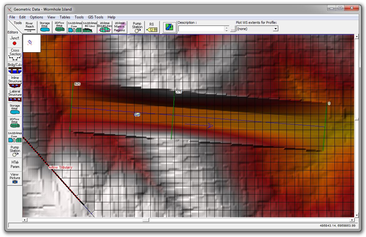
[I have plenty of real examples where I have run up against this limitation, but most of those are proprietary to individual clients, so I’ve created my own example here using the publicly available ELVIS terrain data. With the original ELVIS topography, I could have actually used the Pac-Man method and sliced the external boundary along the ridge line shown in white below – avoiding any 2D flow paths – to get to the internal inflow location; I wanted to use an island for this example, though, so I made my own using terrain modification. To excavate a channel through the terrain, I cut a 1D cross section on each side of the ridge line as shown below, and then generated a new terrain surface using the interpolated channel between the cross sections; this allows the flow to split downstream of the inflow location, forming an island.]
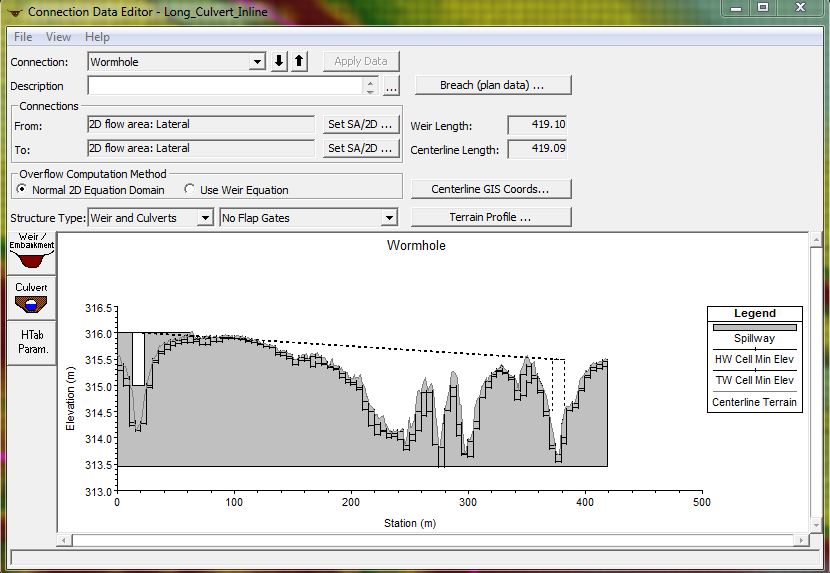
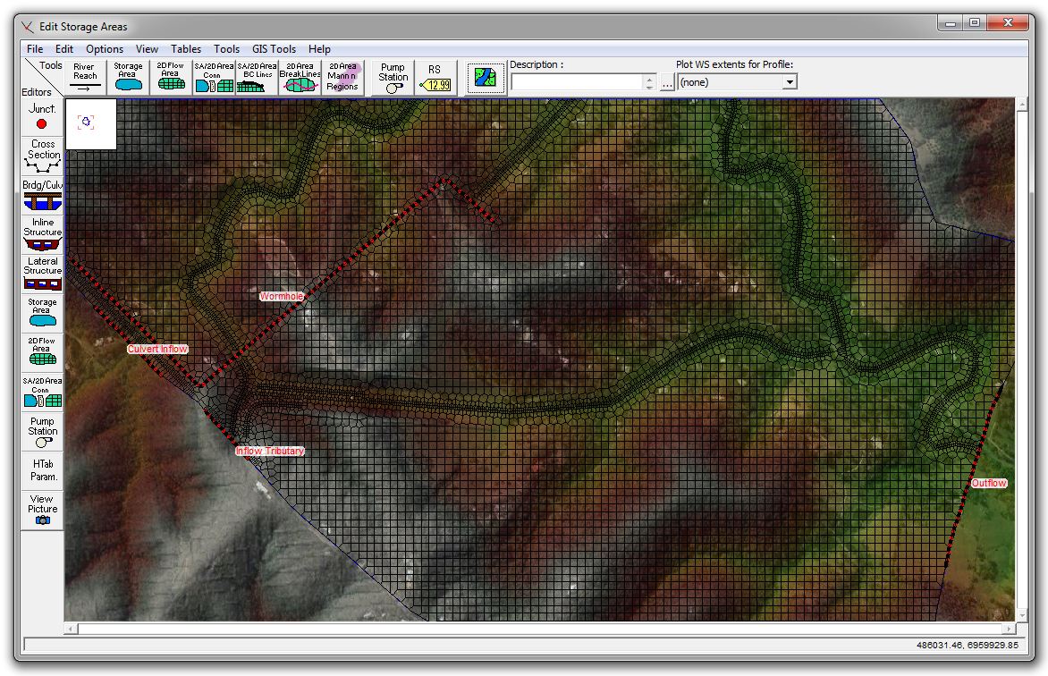
As in the first example above, I then created a dam against the external boundary of the 2D Flow Area using an SA/2D Area Connection, extending the line to the desired inflow location inside the island. It is important that the artificial dam is located far enough away from the area of interest to avoid affecting any other results. If you are trying to apply a specific hydrograph at the internal inflow location, it is also important that the dam is located close enough to the external boundary to keep the storage volume in the reservoir negligible relative to the inflow hydrograph. Here is the schematic plan view of the wormhole culvert alignment with breaklines enforced along each channel centerline:
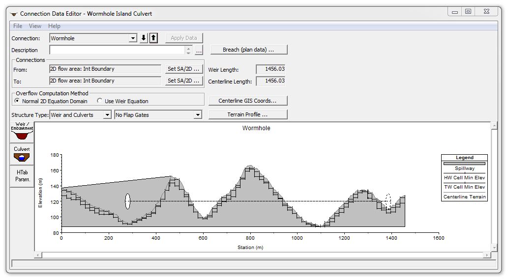
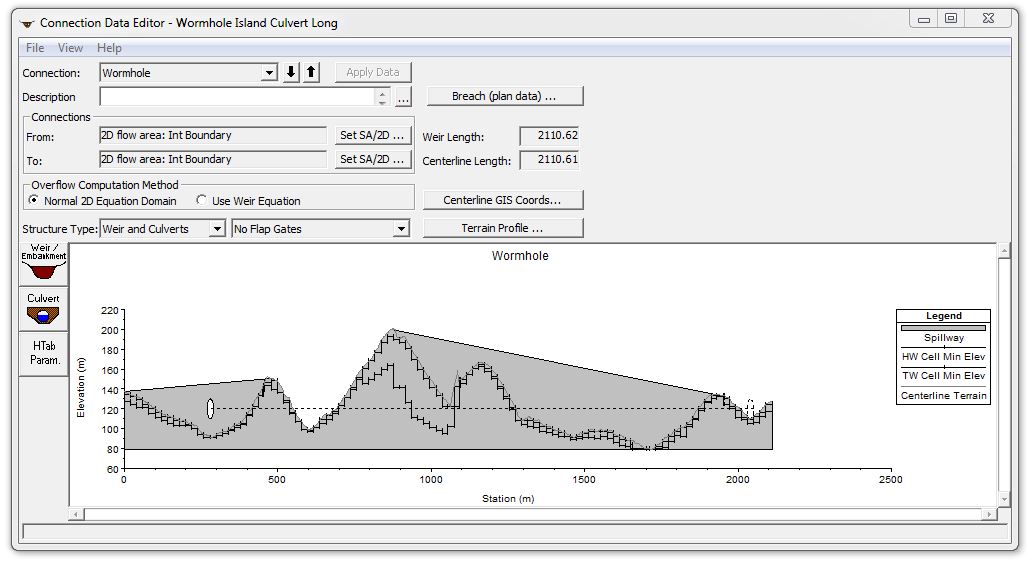
For this case, I’ve made a massive culvert (20m in diameter) with an extremely short length (1m) so that culvert does not affect the hydrograph as it is transferred from the external boundary to the internal inflow location. I copied and pasted the terrain profile to the weir/embankment station/elevation table so that the weir essentially becomes just a line painted on the ground, with no hydraulic effect whatsoever. “Normal 2D Equation Domain” should be selected for this case instead of the weir equation, making the weir width irrelevant to the hydraulic computations. I then raised the embankment adjacent to the inflow location by deleting the intermediate station/elevation points from the table. This essentially forms a dam that prevents any flow from traveling downstream in this location, avoiding hydraulic impacts to the rest of my model. Wherever the connection line crosses a flow path, I have to be sure to follow the terrain at ground level to avoid obstructing the flow. Here is the weir/embankment alignment showing the relative location of the culvert inlet and outlet:
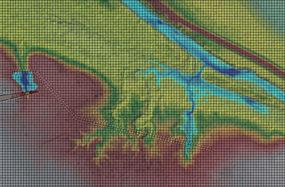
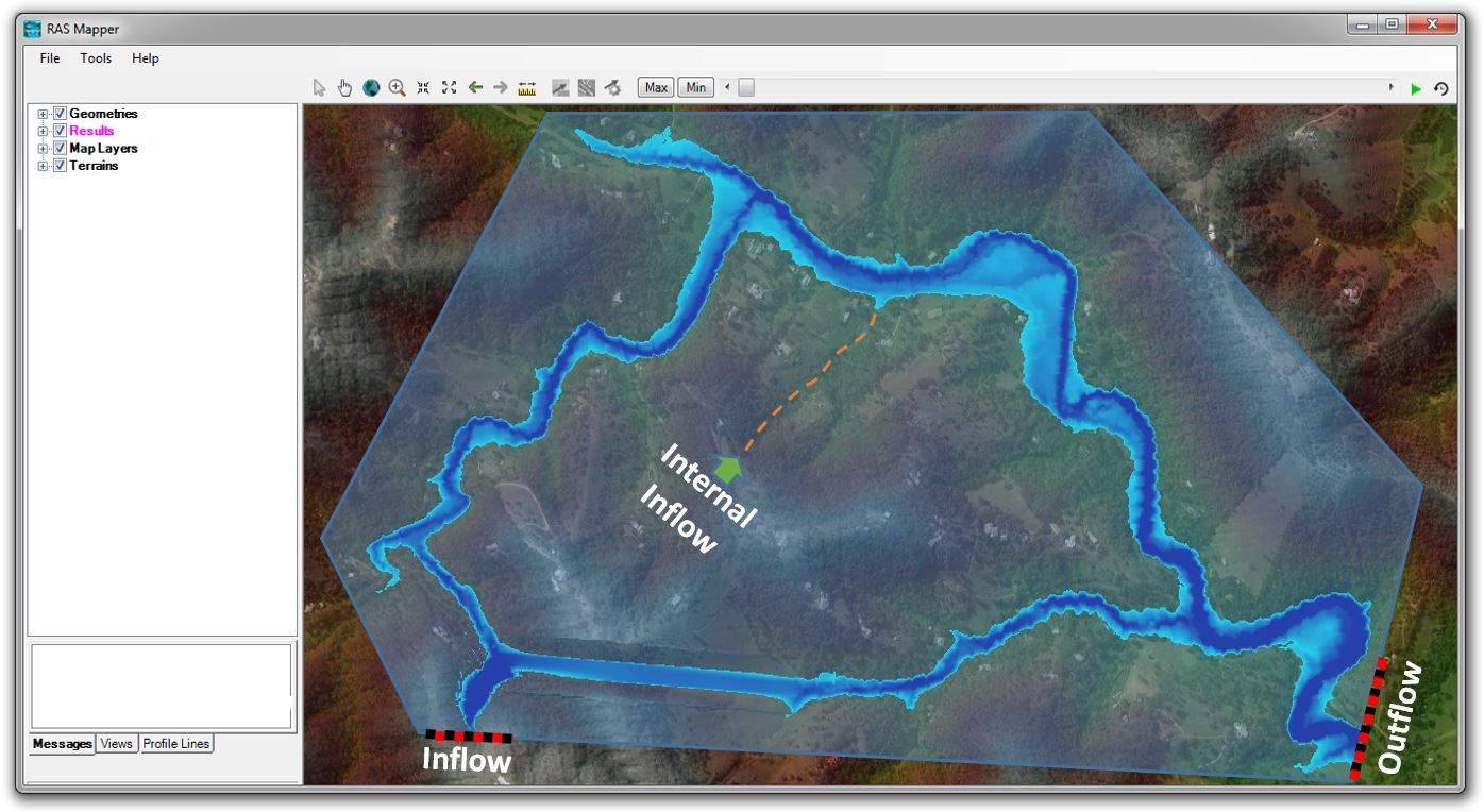
Once I run the unsteady flow plan and animate it in RAS Mapper, I can see the tributary flow appearing at the center without affecting the hydraulics of the “moat” around Wormhole Island:
Although the connection is several kilometers long, the flow appears instantly at the internal inflow location as soon as the water surface elevation in the artificial reservoir reaches the invert elevation of the culvert inlet. [If this were a real project, I’d take it a bit further by moving the artificial reservoir further away so it doesn’t show up in the floodplain maps.] Here’s how the reservoir looks without the structures or boundary condition lines:

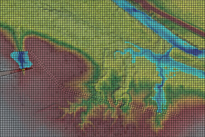
Now back to the whole point of this exercise, I wanted to demonstrate that the alignment of the SA/2D Area Connection (whether it’s a “Z”, “S”, or any other shape) is absolutely irrelevant to the hydraulics. To test the sensitivity, I added a few vertices to the line and moved them around to increase the length as shown here:

Here is the new weir/embankment profile, showing that we have added almost 700 metres to the connection length:
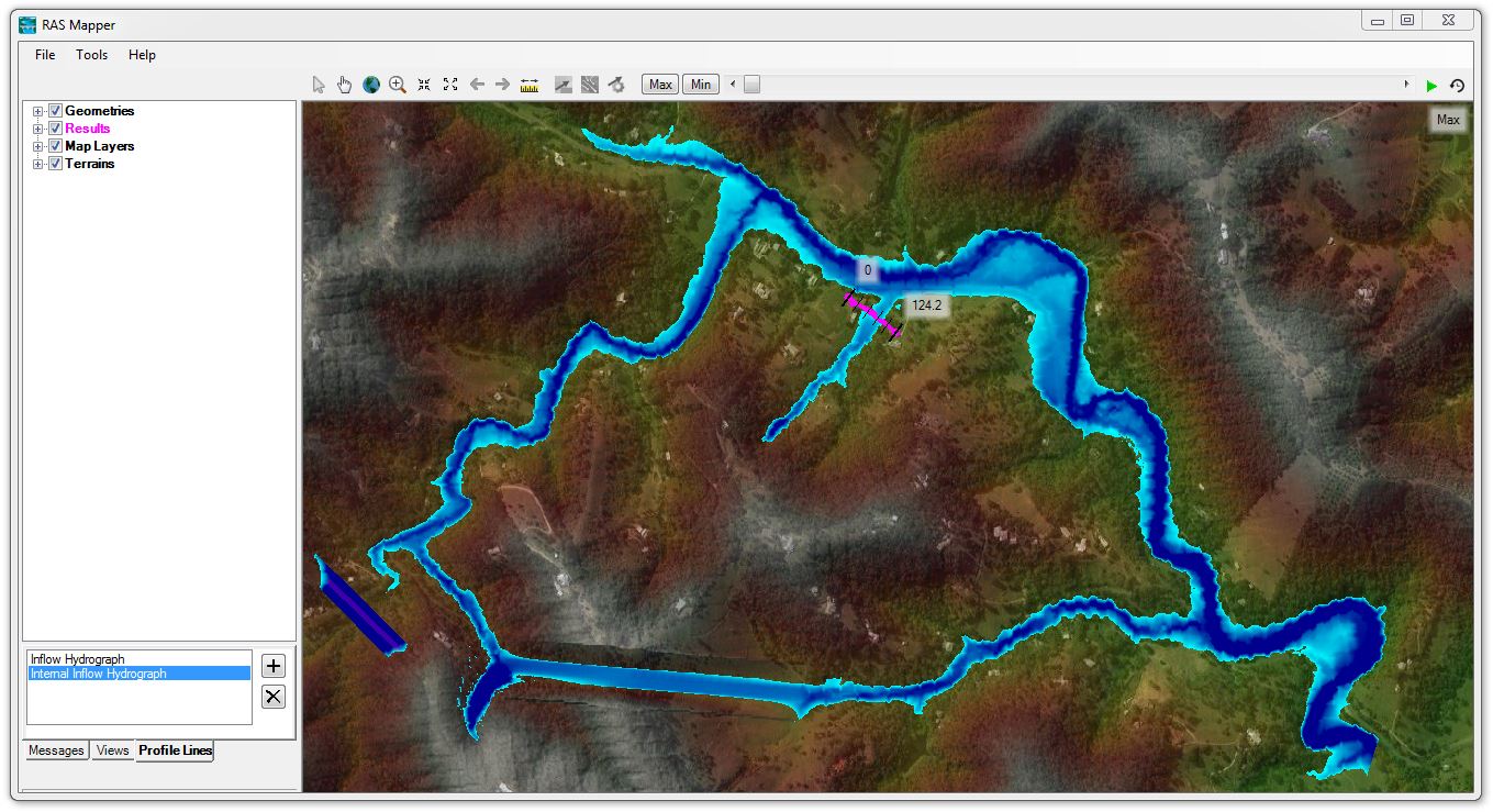
When I run it again, the plan view depth map in RAS Mapper looks identical to the previous run. Just to be sure, I added some profile lines to check the flow hydrographs in the inflow reservoir and in the internal tributary:
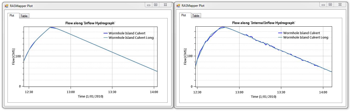
Here are the hydrographs in the reservoir and in the internal channel for both the original wormhole alignment and the extended alignment:
Conclusions
As shown in the hydrographs, the peak flow rates between the inlet and outlet match within less than 1%, and the time to peak is nearly identical, indicating that the wormhole culvert has not affected the inflow hydrology along its path. Likewise the hydrographs from the original alignment match those from the extended alignment, confirming that the length and the trajectory of the alignment are both irrelevant.
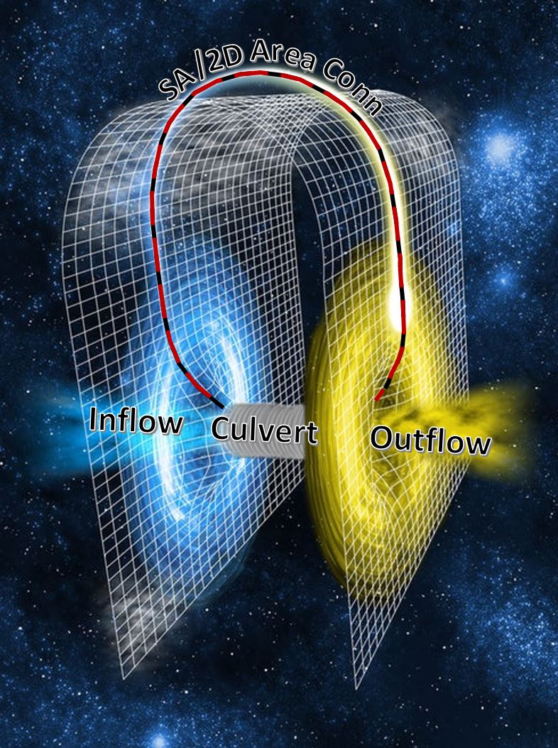
This illustrates why we call them “wormhole” culverts. In our case, flow has traveled several kilometers in no time at all!
I often find myself with a series of nodes at which I need to introduce inflows that have been generated by a hydrological model. These nodes are very rarely located conveniently along the external boundary of my 2D Flow Area! Whether the hydrographs are generated from the Rational Method, RORB, HMS, or any other rainfall-runoff approach, the wormhole method allows us to introduce inflow hydrographs wherever we want to place them, without having to adjust the boundary of the 2D Flow Area. Using multiple, interconnected 2D Flow Areas gets a bit more complicated but opens up a few other possibilities as well – I think I’ve rambled on enough for today, though, so I’ll have to cover that topic in a future post!
[Disclaimer: Although I have confirmed the hydrology for this particular case, I wouldn’t apply these findings to any other model without checking the results first. Flow that is essentially introduced as a point source like a culvert may behave very differently near the source area than flow that is distributed along a selected cross section. By comparing the original inflow hydrograph to time series that are extracted along key profile lines throughout the hydraulic model, you may find some issues that need resolving; if I needed to limit the peak flow attenuation or lag time in my model even further, for example, I could reduce the volume of the artificial storage reservoir by moving the SA/2D Area Connection alignment even closer to the inflow boundary condition. I could also take it a bit further and tweak my time steps or other parameters to reduce the instabilities that resulted in some of the minor oscillations apparent in the hydrographs; for the purpose of this example, however, I think we’ve sufficiently made the case for wormhole culverts!]
Read more:
- Wormhole Culverts Part 1: Introducing the wormhole concept
- Wormhole Culverts Part 2: Using wormhole culverts for internal boundary conditions
- Wormhole Culverts Part 3: Comparing wormhole culverts to 1D/2D bridges and culverts
- Wormhole Culverts Part 4: Sensitivity analyses for wormhole culverts
- Wormhole Culverts Part 5: What’s the best shape for a wormhole culvert?
Contact and feedback:
- Please e-mail me any comments or questions about wormhole culverts or other topics
- Contribute to the discussion about wormhole culverts on the RAS Solution blog
- Subscribe to receive updates when new content is published
- Join the newly created LinkedIn groups for dam break modelling and sediment transport modeling
Krey Price
Surface Water Solutions