
Rating Curves Part 4: Sensitivity Analyses
Please visit our updated Rating Curves article at hydroschool.org/rating/.
All continuing education resources previously listed at surfacewater.biz have moved to hydroschool.org; going forward, the surfacewater.biz website will be dedicated to drainage-related consulting work only.
Below is the archived version of the rating curves article.
Welcome to our four-part series of articles about rating curves:
- Rating Curves Part 1: Webinar recording and background resources
- Rating Curves Part 2: What is a rating curve?
- Rating Curves Part 3: Extracting flow and stage results from a 2D model
- Rating Curves Part 4: Sensitivity analyses
Optimising Gauging Locations
Now let’s have a look at how the rating curve changes along the channel, which might be a useful exercise if we were trying to select an optimal gauging site. Here are three optional locations for our make-believe gauge:
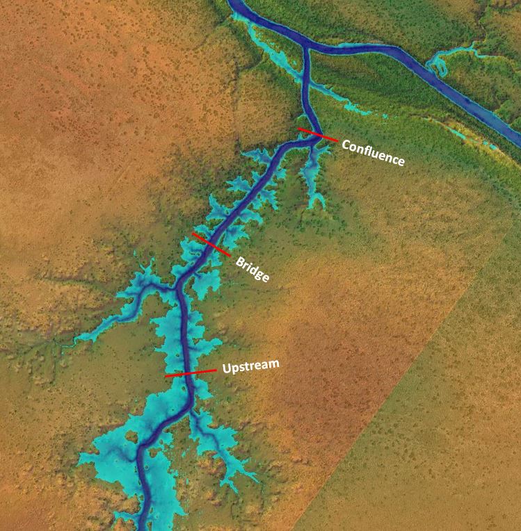
Following the same steps as described above, we can develop flow and stage hydrographs along with rating curves for the three locations. This particular run has one inflow hydrograph entering the tributary with very low flow in the main channel to avoid backwater effects from the confluence. Here are the resulting charts:
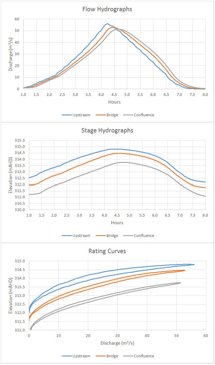
The flow attenuation is apparent from the hydrographs as the flood wave moves downstream. As shown in the charts, the looping effect varies with the amount of storage in the downstream floodplain. Even though the flow is generally contained in the channel for each of the cross section locations shown in the plan view, if you look closely at the floodplain extents downstream of each site, the upstream site has the most floodplain storage and exhibits the largest looping effect while the downstream site has the least floodplain storage and exhibits the smallest looping effect.
We can also vary the amount of looping by adjusting the shape of the hydrograph as discussed here. If flow could actually be measured in these locations, we may find that individual events can each have a unique rating curve pattern. We may be tempted to choose the site with the least looping so that a single discharge value could be assigned to each stage, but we’ll need to check a few additional factors first.
If you wanted to gauge your tributary to estimate the volume contribution or rainfall-runoff relationships, you would want to capture as much of the catchment area as possible. But you also want to stay out of the backwater area near the confluence, so we are faced with a bit of a trade-off here.
Effect of structures
It’s generally most practical to measure flow rates at a structure where the flow is confined, but the structure itself can significantly complicate the rating curve. Let’s have a look at the impact by adding a structure to our model. For this exercise, I’ll lift the terrain to represent roadway fill in the floodplain and a bridge structure across the channel. I’ll do this by adding a 1D reach with cross sections representing the roadway. See the article on terrain modification for some links and examples of how to do this. Here is the “orphan” geometry (not combined with any flow) showing the 1D reach for generating a new terrain file:
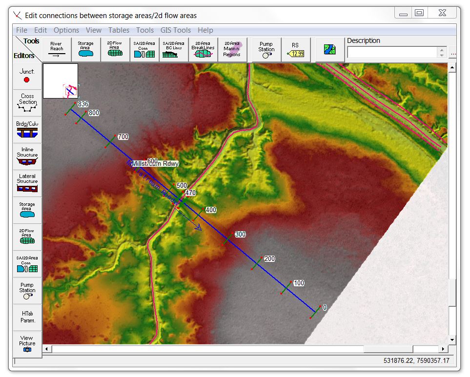
For this exercise, I want to see how both pressure flow and overtopping flow affect the rating curve, so I’ve set the deck elevations low enough to allow some overtopping and engage the floodway during peak flood conditions. [These screenshots show the now obsolete wormhole culvert method to account for both the structure and the terrain in the 2D model]
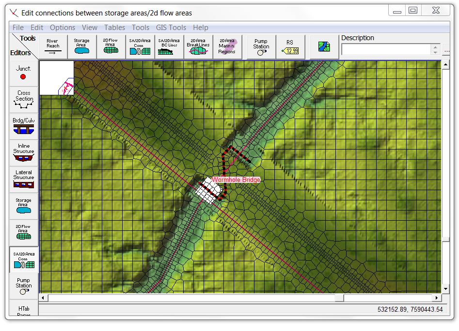
Here’s how it looks in RAS Mapper just before overtopping:
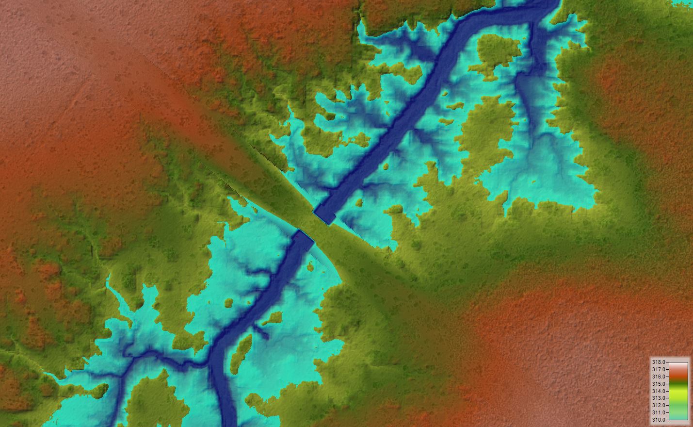
Depth-averaged hydraulic models won’t necessarily provide an accurate distribution between weir flow over the road deck and pressure flow through the culvert, but let’s see how that situation affects the rating curve.
I’ll make a few other changes to this run to make it look a bit more realistic and less like a textbook chart:
- I’ve shortened the hydrograph to be more representative of actual flow conditions and response time in this catchment. The system is relatively “flashy”, and the timing of the flood wave arrival doesn’t typically allow for the establishment of normal depth conditions during the rising limb.
- I’ve also put a typical flood flow in the mainstem channel to see whether the sites follow a backwater/tailwater curve during the rising or falling limbs.
Here are the resulting hydrographs and rating curves:
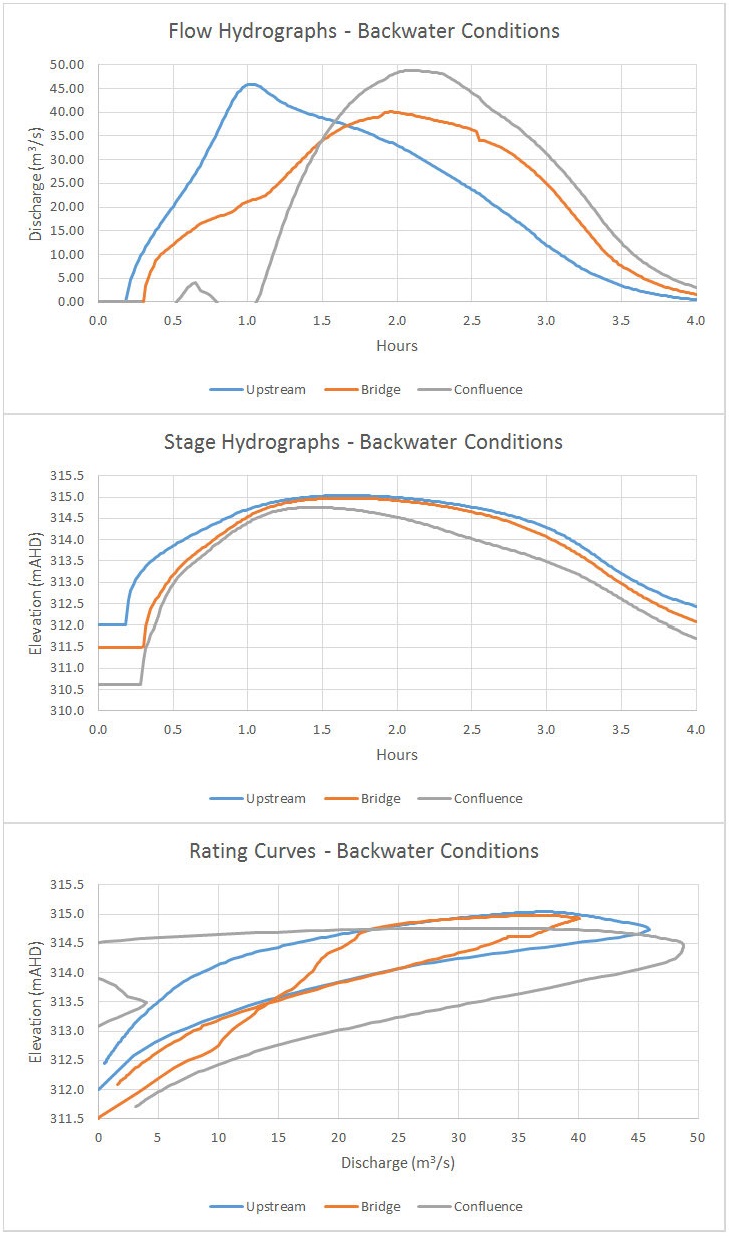
As indicated by the charts, shortening the hydrograph duration significantly increases the observable looping on the rating curve. In addition, the backwater effect from the mainstem confluence and/or the bridge affects all of the sites, further contributing to the magnitude of the looping effect. Here are a few observations for the individual sites:
- Upstream Gauge. The highest peak flow does not coincide with the highest stage, indicating that the backwater from the bridge is still pushing up the water surface well after the peak flow has passed that point.
- Bridge Gauge. The highest peak flow occurs roughly at the same time as the highest stage. The effect of the bridge itself can be seen by the distinct inflection points, particularly during the rising limb where flow is initially pressurised with inlet control but eventually changes to outlet control from the downstream backwater.
- Confluence Gauge. The net flux across the gauge is negative at times, indicating that the mainstem river is actually pushing flow upstream. The tailwater effect is massive here, since the stage is still high due to the mainstem flow even after the tributary flow has receded.
The bridge site might be a tempting place to put a gauge, and you might do just fine if you’re only interested in peak flows. But if you are interested in using the data to estimate the volume of water that passes through the bridge during a storm event (essentially integrating the hydrograph by taking the area under the curve) the results will likely be highly inaccurate.
Direct Rainfall
The above examples assume that the only available flow comes from the main channel. That flow then fills the minor tributaries as the flood rises. In reality, some of these tributaries would be fed by localised sheet flow during the same rainfall event. To make things a bit more realistic for a small catchment in which the precipitation fills storage areas, we can apply a direct rainfall model. I’ve adjusted the rainfall rates to provide roughly the same outflow for the tributary as in the models above. Here is a screen shot from RAS Mapper showing the direct rainfall results:
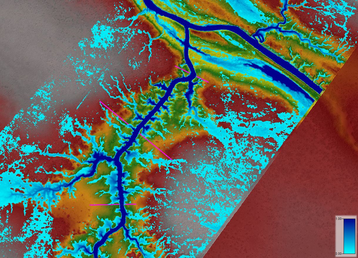
Here are the resulting hydrographs and rating curves for the three gauging locations:
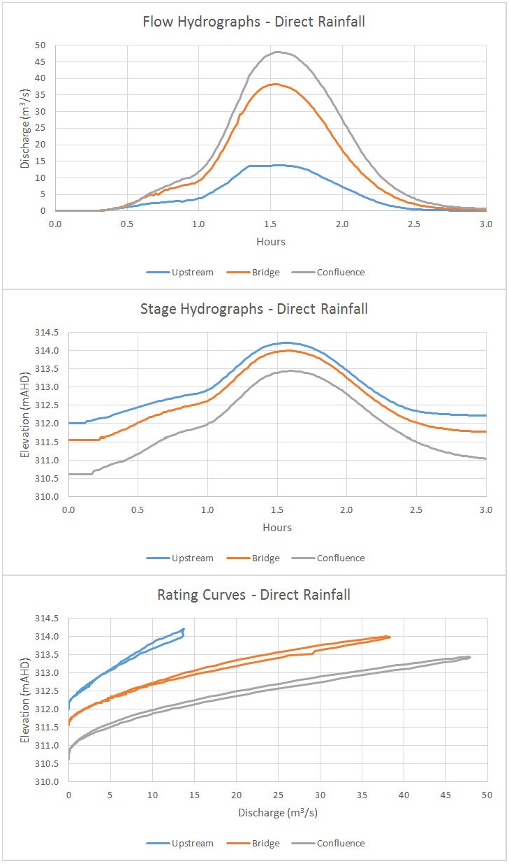
Note that the degree of looping is significantly lower since some of the floodplain storage area is already inundated by the time the peak flow passes along the main channel.
Roughness sensitivity
A roughness sensitivity should accompany any hydraulic model. If we are unsure of our roughness coefficient (and we always are), the roughness coefficient sensitivity analysis can quantify the potential variation. The above models use the default Mannings roughness value of 0.06 as the base case. For the sensitivity runs, I used a range of 0.04 on the low end to 0.08 on the high end.
These models do not include spatially varying roughness coefficients, which we could add if aerial photos or ground photos showed distinct differences in different zones. Keep in mind, though, that HEC-RAS does not currently allow for depth-varying roughness; the effect of depth-varying roughness coefficients for a model like this with significant overbank flow can exceed the effect of spatially-varying or even seasonally varying roughness values.
Here are the hydrographs and rating curves for the roughness sensitivity:
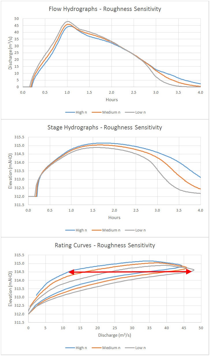
As shown in the stage hydrographs, the peak flow rates match much more closely than the stages during the falling limb.
Although the both the peak flow rates and peak flow depths for the high and low roughness sensitivity runs match the results of the medium run to within +/- 5%, the rating curve exhibits a much wider range of variability. As shown in the curves above, for instance, a river stage of 314.5 m could correspond to discharge rates ranging anywhere from 12 to 47 m3/s, or the equivalent of a +/- 50% variation from the medium value.
Even when roughness coefficients have been calibrated, bushfires, debris, seasonal vegetation changes and other factors can have a tremendous effect on the rating curve. Given the large effect that a perfectly realistic range of roughness coefficients can have on the results, it might be worth presenting results in terms of a range rather than absolute values.
Time step sensitivity
Sometimes it’s not practical to meet the recommended Courant Number criteria at every computation point at every time step. (Search for “Courant number” in the 2D manual for a reference). If we can’t meet the recommended criteria, we at least need to check the model for stability. A time step sensitivity test is one way to ensure the results have reached convergence.
The above models all use a time step of 5 seconds. If I go down to my smallest grids (1 metre) and take my highest velocity (4 m/s…or 8 if you add wave celerity) I would need time steps of 0.1 seconds or so. This would significantly increase the run times. But would I get any benefit out of the change?
In order to check, let’s be sure to break our model first by using a completely unreasonable time step along with some intermediate values and see if we get convergence. Here is a plan view taken from the same point in time for a 30-second, 10-second, and 5-second computational time step:
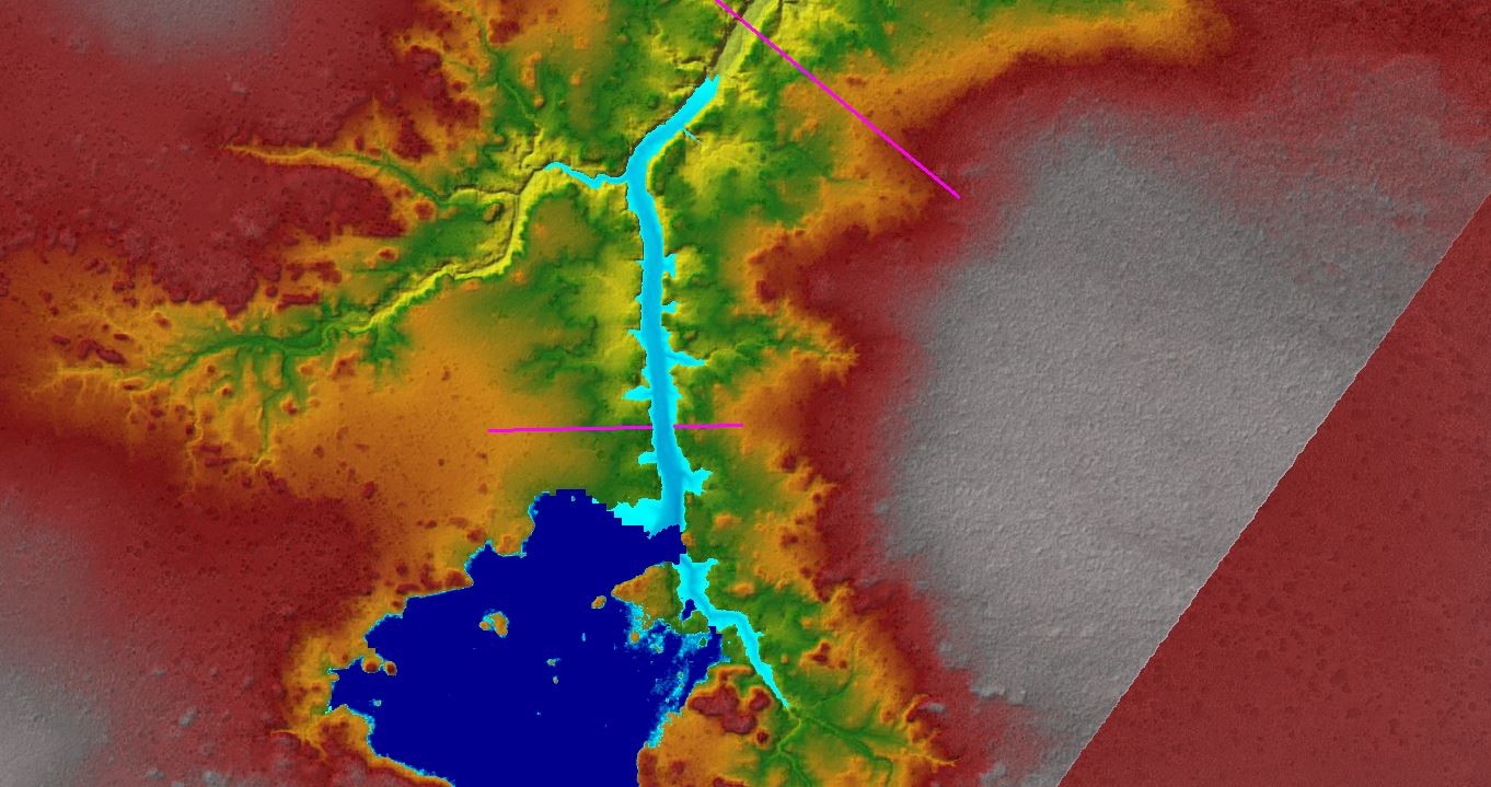
The dark blue area shows the inundation extent for the 30-second result. The other two extents are indistinguishable from each other. What we see in dark blue is the typical evidence of a severe Courant Number infraction: The flood wave extends in a straight line from bank to bank and does not fill the low flow channel as it proceeds downstream. This is easier to visualise with a WSE profile plot:
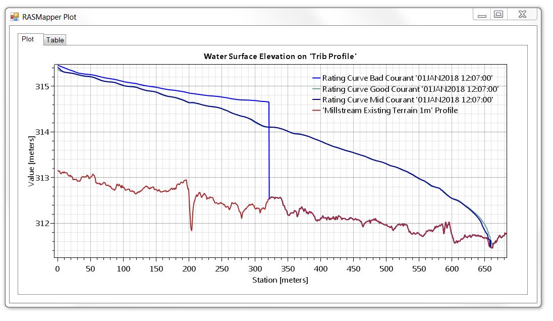
The three profiles are taken from the same time step in RAS Mapper. The only change between these runs is the computational time step; all other geometric data and flow data remain the same.
As shown in the profile, the wetting front for our 30-second time step model can’t keep up with itself (a water particle would have travelled over many grids from one computation to the next). As a result, the wetting front is computed as a vertical wall of water. In some models this can produce unreasonably high water surface elevations that would require more water than is available from the inflow hydrographs! As you can see, any predicted arrival times would be way off.
Both the 10-second and 5-second runs give us a nice smooth wetting front, however, which is what we want to see. Because the 10-second and 5-second run profiles are essentially identical, we can be fairly confident that the results are converging. It might be worth trying a shorter run using a time step of, say, 2-seconds, just to confirm, but I’ll leave it there for now.
Here’s how the time step affects the hydrographs and rating curves:
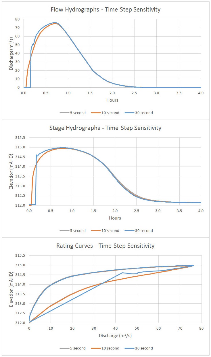
As you can see, the peak flow is essentially unaffected along with the entire falling limb, but the rising limb is where the highest velocities (and thus the worst Courant Number violations) occur. Looking at the 30-second model, we’ll throw that one out. The 10-second and 5-second rating curves are essentially identical, so we have confirmed convergence and could probably get by using either one.
Additional sensitivities
Several other variables could be adjusted as a sensitivity analysis. We won’t cover them all in detail here, but the equation set it probably worth mentioning. All of these runs use the Full Momentum equations set that best accounts for acceleration terms. If run times were an issue, switching the plan files back to the default Diffusion Wave simplification may be acceptable, but only if a sensitivity analysis has shown that the inertial terms are not critical to your results.
For relatively small models where the gauge location is fairly close to the external boundary conditions, you may also wish to tweak the EG values for the upstream and downstream boundary conditions to check the sensitivity and make sure we’re outside any significant zone of influence. Selection of the optimal gauge location can be greatly aided by 2D modelling results before heading into the field to install a gauge. If the stage-discharge relationship changes significantly over time, the installation of a second gauge upstream or downstream may be warranted. This can provide a reality check on the longitudinal slope, which can then be used to develop a series of rating curves based on the slope. Programming these calculations and post-processing the collected data can be more complicated, but this can provide much more realistic results. If you have budget for two gauges, sometimes you’re better off putting them near each other and getting meaningful results at a single site rather than putting them farther apart and getting bogus results at two sites!
Caution
If you try to extract stage and flow hydrograph data from third-party software (QGIS, Waterride, etc.) for use in a rating curve, your results may be very different. In order to check the validity of your results, try drawing your cross section at different angles and check the hydrograph. As long as your section line spans from one dry bank to another on the opposite side, the angle of your section line should not affect the net flux through that line significantly.
Even moving the cross section 100 metres upstream or downstream of your gauge shouldn’t affect the flow much; as long as you haven’t picked up some tributary flow or split flow in between, the peak flow rate and the total flow volume should match fairly closely. Even when reality and intuition tell you it has to be the same, however, some programs can give you wildly different flow volumes and peak flow rates depending on the orientation of your cross section. This may have to do with how velocity vectors are calculated at face points with areas measured along cell faces that don’t line up with the cross section line. I haven’t investigated this in detail, but I have seen erroneous results come out of third-party viewers. For this reason, I recommend only extracting hydrograph values from the source program and not from other viewers.
Calibration
So far we have only addressed the extraction of rating curves from hydraulic models. In many cases, rating curves are developed straight from measurements.
The resources in Part 1 include a number of publications that highlight the complexity of collecting accurate field data and then mathematically fitting the acquired data using functions that provide the best reflection of the system. If any actual flow measurements are available with their corresponding stage, roughness values or other parameters can be adjusted in the hydraulic models to try to get the simulated rating curve to match the calibration point on the chart. Getting a curve to match a single calibration point is relatively straight-forward; however, getting a curve to match the measurements at multiple points using the same geometry file can be a bit more challenging (especially when using HEC-RAS, which does not currently allow depth-varying roughness coefficients, requiring the use of constant values over time – here’s a quick hack in the meantime).
With the roughness or other calibration variables adjusted to match the measured points as closely as possible, the model results can be used to interpolate or extrapolate the remaining values. Extrapolations need to be treated very cautiously and should always be appropriately caveated as such!
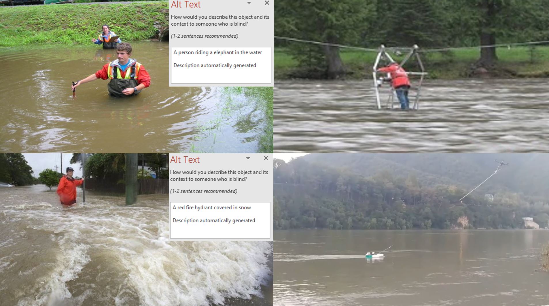
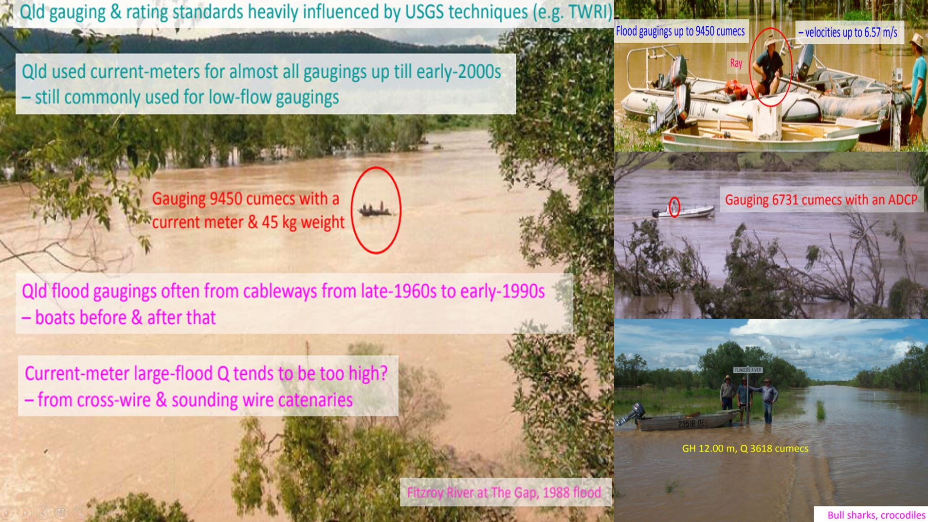
[At least in Western Australia, safety concerns often prevent anyone from taking flow measurements during peak flow conditions (usually during tropical cyclones!) so high flow are almost always extrapolated from lower measurements. See Ray Maynard’s presentation in Part 1 with references to crocs and bull sharks – Safety First!]
Summary
I have recently been working on hundreds of rating curves using 2D HEC-RAS models as part of some efforts to establish confidence bands at existing gauging stations. The findings are sometimes a bit shocking: the flow rates that we assume are occurring when the river is at a particular stage can vary dramatically between modelling approaches, especially in “flashy” systems. And the predicted flow volumes derived from those relationships are often entirely hopeless, sometimes varying by an order of magnitude or more from actual measurements. This is especially the case during receding conditions when there is very little flow – or even no flow at all – associated with a stage that, according to the rating curve, should correspond to a significant flow rate. The formation of a downstream sediment bar or other obstruction, for example, could give the false impression that flowing water is being provided to downstream sources when in reality the water is just ponded.
Rating curves derived from 1D steady flow models, 1D unsteady models, and 2D models can exhibit extreme variation; all are of course reliant on current, accurate survey data which often isn’t available, particularly for mobile beds with substantial sediment movement. In some cases, changes in morphology can introduce larger discrepancies to the rating curves than the modelling approach itself. Changes in seasonal roughness add further uncertainties that typically aren’t accounted for in the application of rating curves to generate flow estimates.
Given the potential differences in results and the relative ease of applying 2D models, it is at least worth checking curves that were previously derived from 1D models or normal depth calculations to determine which ones can continue to rely on previously developed relationships and which ones need to be revisited and potentially recalibrated with measured flows.
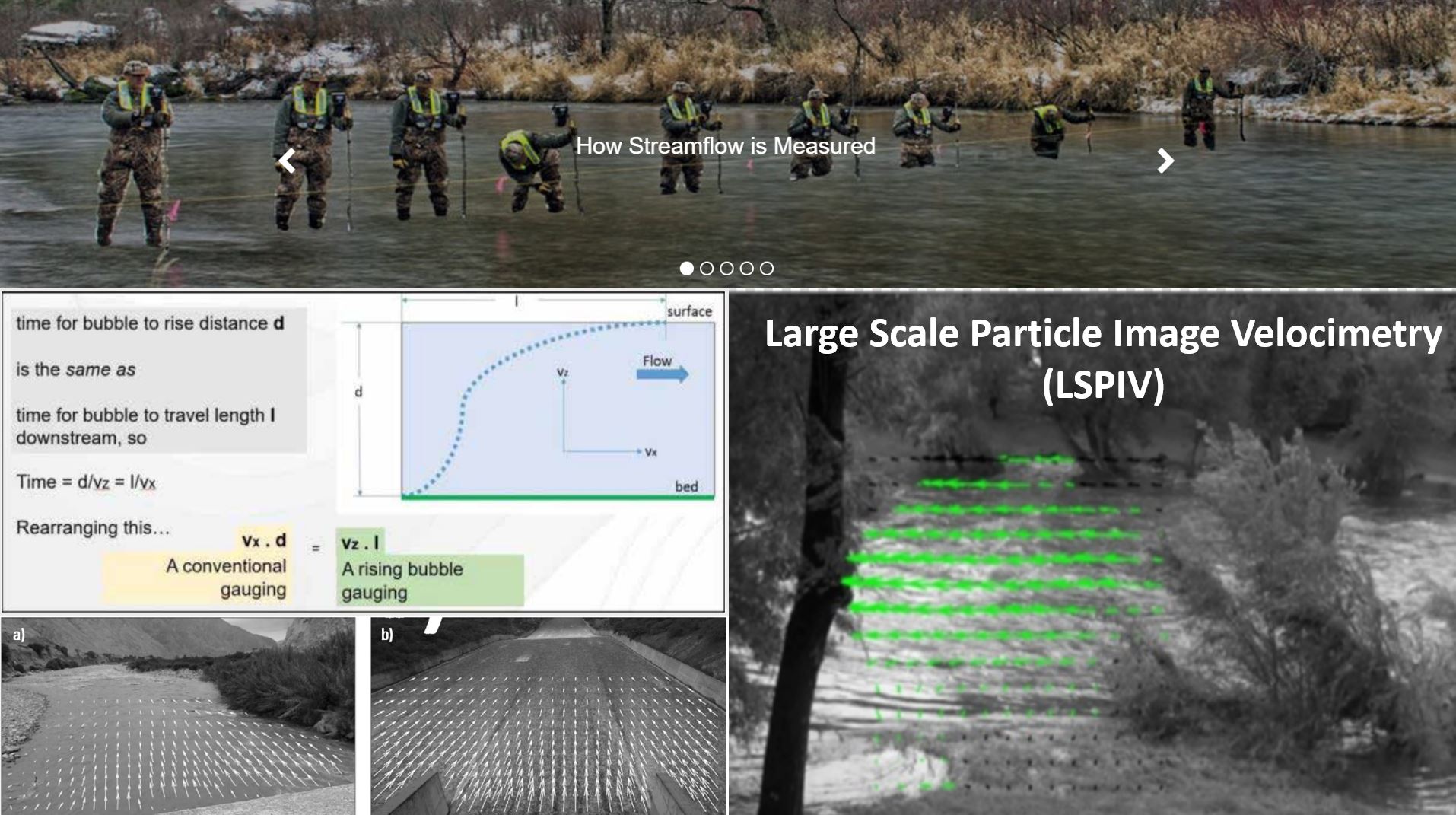
There are some exciting new innovations on the horizon that will improve our ability to better imitate Mother Nature, both with software (like the incorporation of wind forces in HEC-RAS 6.0 which can significantly affect stages and thus the rating curves as well) and in terms of equipment and methodologies (such as the use of LSPIV, bubble methods, drones, etc.)
Watch our webinar in Part 1 for a presentation and panel discussion on the latest advances in the development of rating curves. If you need help with project scoping, model setup, or even developing a customised program to set consistent protocol for stream gauging, please contact me.
Krey Price
Surface Water Solutions
Read the rest of our articles about rating curves:
- Rating Curves Part 1: Webinar recording and background resources
- Rating Curves Part 2: What is a rating curve?
- Rating Curves Part 3: Extracting flow and stage results from a 2D model
- Rating Curves Part 4: Sensitivity analyses