Making Middle Zealand – Surface Water Solutions: Consulting and Software Training

This article covers terrain modification in HEC-RAS and the introduction of tidal boundary conditions as stage hydrographs. For this example (Workshop #6 from our New Zealand course), we’ll set up one of our tutorial models from scratch and create a new island that we’ll call “Middle Zealand!”

[By the way, all of the data sources for this model are freely downloadable, so if you want to try this for yourself, go ahead and follow along!]

A Slice of Northland

As I was trying to navigate my way across New Zealand’s North Island a few months ago, I was surprised to find that the only thing keeping New Zealand’s two main islands from being three separate islands is a little 2 km stretch of land in Otahuhu just south of Auckland. If you were to excavate a canal across that narrow strip, it would connect Mangere Inlet on the west with Hauraki Gulf on the east, shaving 800 km off the sea voyage around Northland in the process:

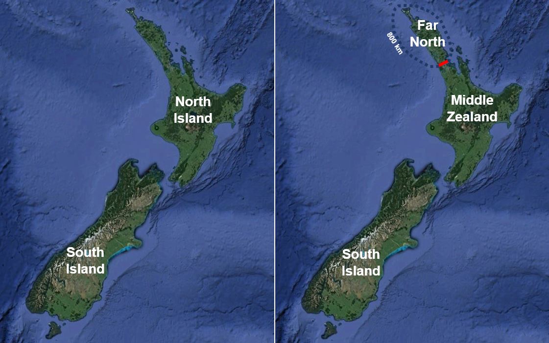
If you went and rented yourself a Bobcat, you could probably excavate the channel single-handedly in less time than some of us have spent working on the latest version of HEC-RAS. So why hasn’t anybody done it yet? Well, for one thing, it would be an ecological disaster (given the mixing of species that is an inherent and unfortunate by-product of many of the world’s canals). You would also need quite a bit of dredging in the bays on either side of the canal to accommodate any significant ship traffic.

Because the tides on the west side of the island are out of phase with the tides to the east, the current through the canal would alternate directions, forming a tidal bore under some circumstances and potentially requiring locks to accommodate navigation. So it’s not quite as simple as it sounds; but I’m always looking for cool case studies to use as course material. So let’s cast all of these issues aside for the moment and have some hypothetical fun with the idea in HEC-RAS!

Here’s a short clip of what we’ll be looking at by the time we finish this exercise:

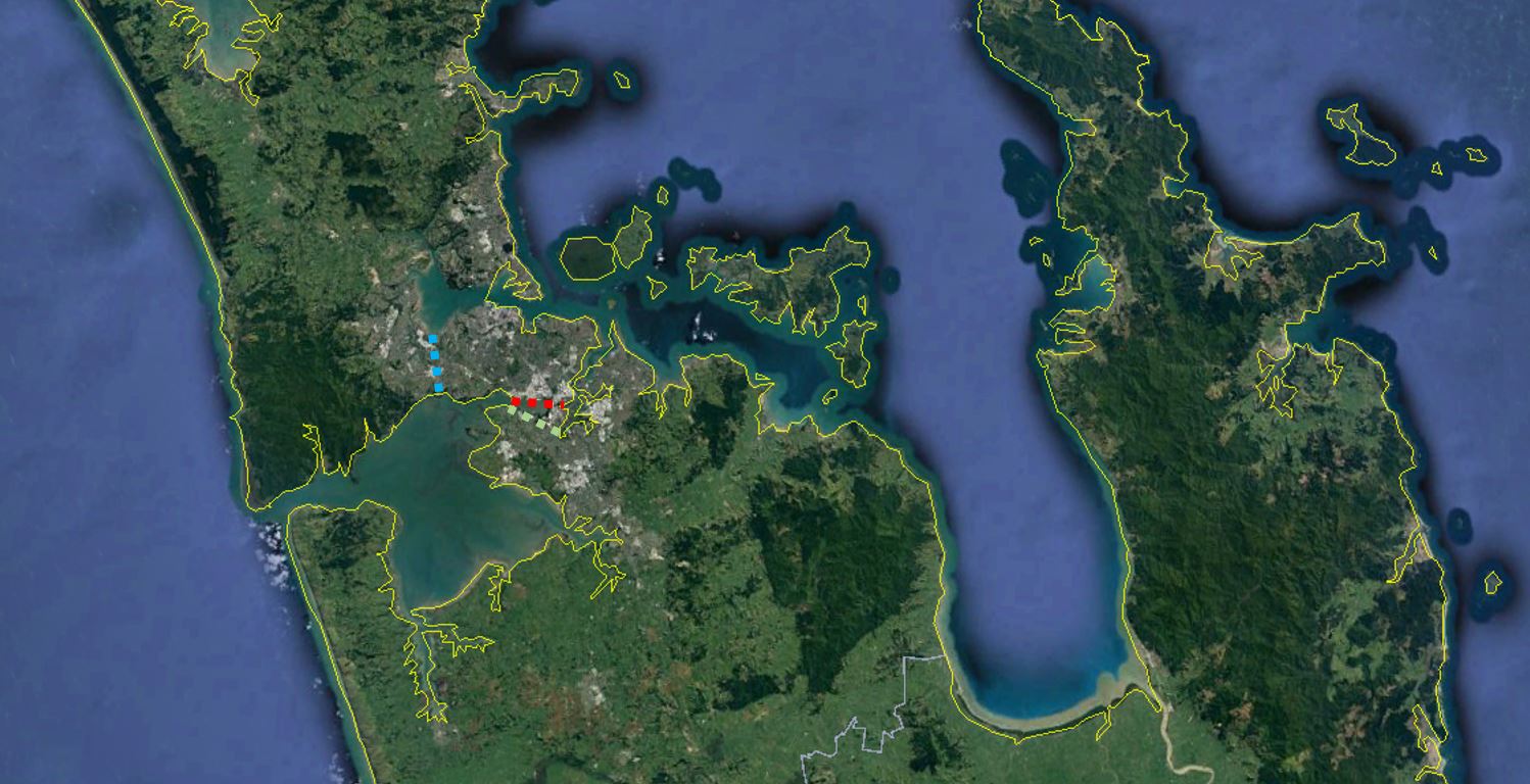
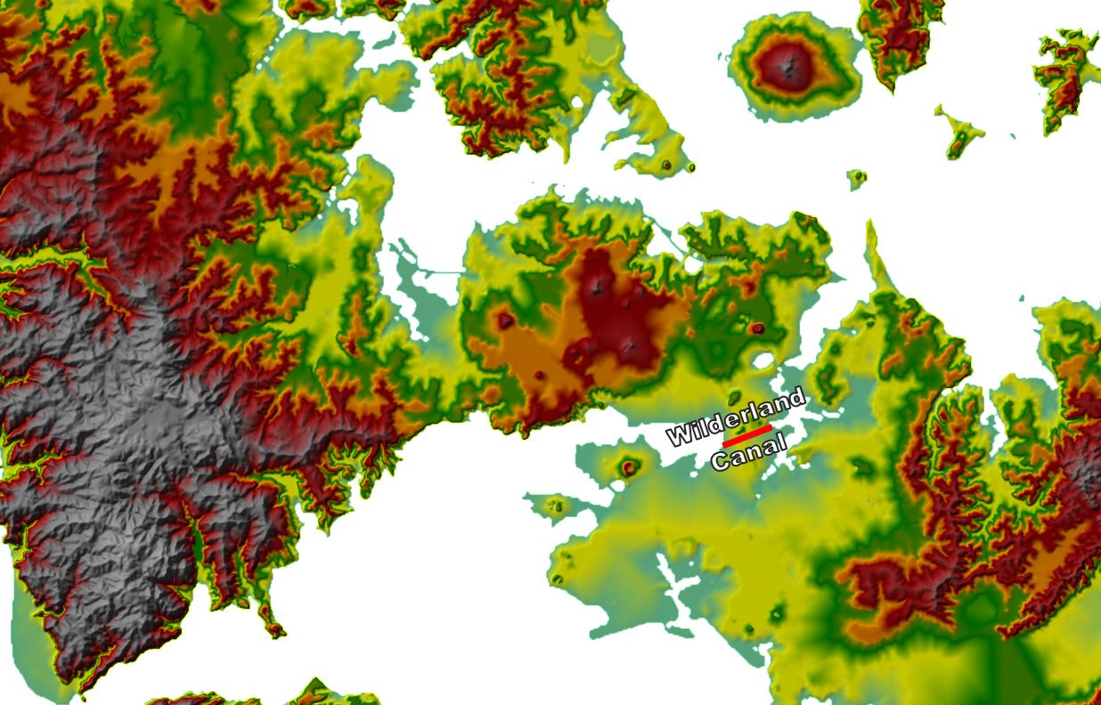
So back to the beginning, the images below show some prospective canal alignments that would sever Northland and half of the Auckland Region from the North Island. While the Southern route shown in green requires the least excavation, the red dashed alignment is the shortest path – following the historical Portage Road.

[Read about the Maori First Fleet’s use of this portage along with previous plans for a canal here. According to the article, Portage Road “must surely be the shortest road between two seas anywhere in the world.”]

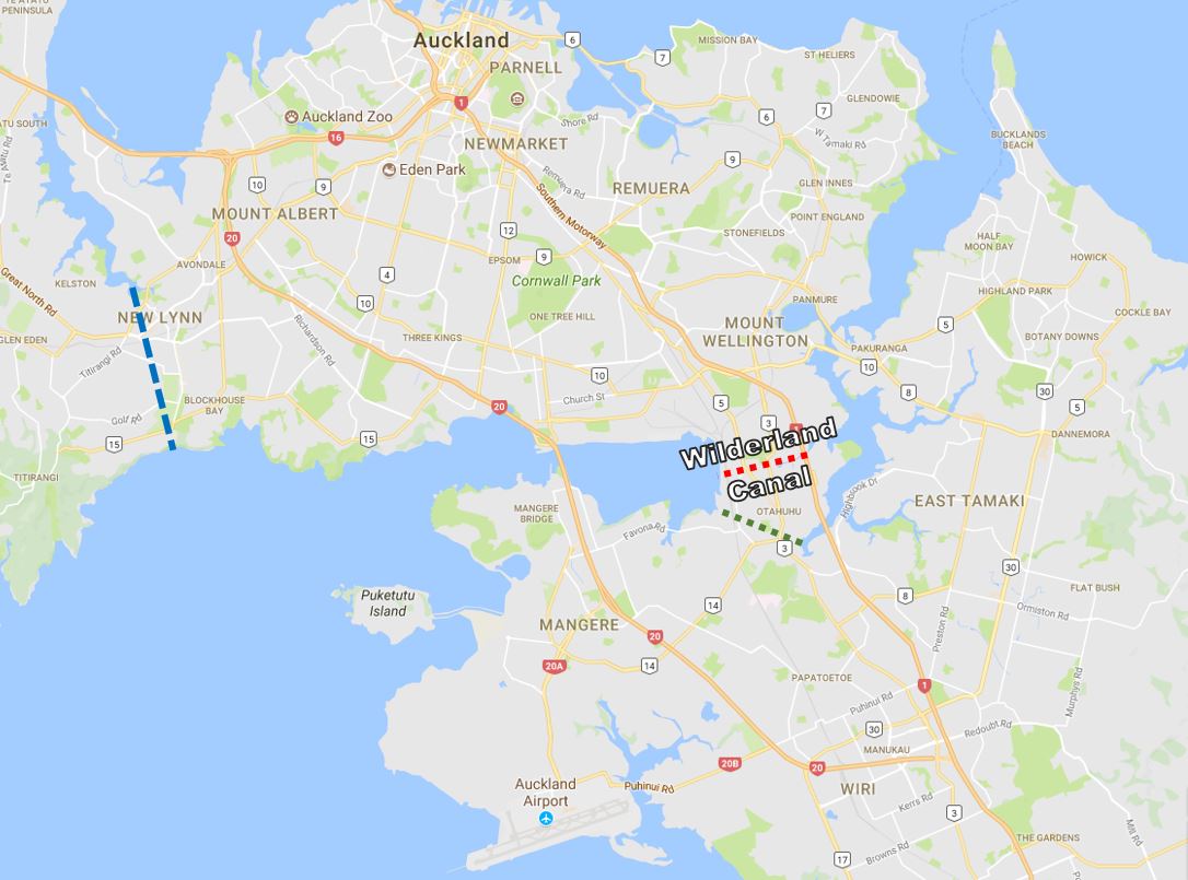
For this write-up I’ve selected the Portage Road alignment; I’ll keep the Middle Earth theme going and call our ambitious new waterway project the Wilderland Canal:

I’ve generally found that course attendees retain concepts best if they do something a bit different than the written example – customising the process rather than walking through the prescribed steps verbatim; so if you’re following along with your own model, feel free to choose your own canal alignment. In fact, you could slice a canal right through the centre of either the North or South Island if you wish; it doesn’t have to be economically or environmentally feasible to take some practice swings!

As a huge disclaimer, please keep in mind that we won’t necessarily be making a robust, hydraulically defensible model of the canal here – the goal is to just walk you through the canal-building process in HEC-RAS as simply as possible. Here’s the approach we’ll follow in ten basic steps:

Compile tidal data for the bays to the east and west
Compile existing terrain data for the region
Create new HEC-RAS project and add geospatial data in RAS Mapper
Add bathymetry to the terrain data
Add the canal to the terrain data
Draw a 2D Flow Area in the Geometry Data Editor
Add boundary condition lines and breaklines to the geometry file
Enter stage hydrographs in the unsteady flow file
Set up and run the unsteady plan file
View and animate the results in RAS Mapper

This shouldn’t have to take up your whole day; most course attendees are actually able to get through the process and animate results for a basic model of the canal in an hour or so. Then once we’ve got the model set up, we can make it more interesting by demonstrating a number of other capabilities in HEC-RAS; some of the next steps we typically take with the completed models in advanced courses include:

add hydraulic structures with culverts or time series-controlled gates in the canal to simulate navigation locks or weirs
put a dam across the canal and breach it to simulate failure of a lock gate or weir
check the water surface differential and examine the feasibility of tapping the tidal energy in the canal with a power plant
add direct rainfall on the surrounding catchments to contribute overland flow to the bays

The list could of course go on and on, but let’s get started with the basics before we get too far ahead of ourselves!

Step 1: Compile Tidal Data

Before we do anything else, let’s grab some tidal data to check the range of water surface elevations that we’ll be working with. If you Google “New Zealand tidal data” the top result will generally be from the Land Information New Zealand (LINZ) tide prediction page. Here’s a screen shot of the website with the interactive map zoomed in on the Auckland area:

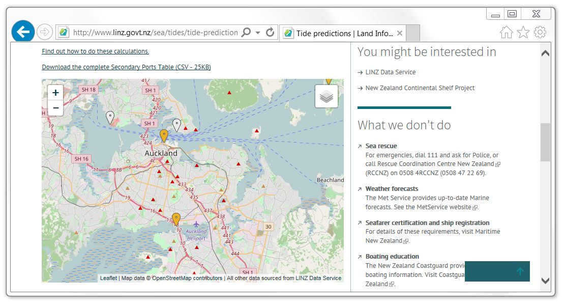
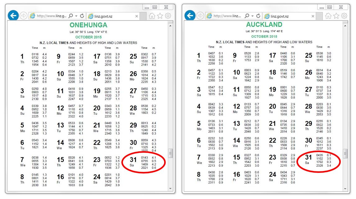
Active tidal gauges are shown with yellow markers. For this exercise I’ll grab tidal data from the Onehunga gauge for the western boundary condition and from the Auckland gauge for the eastern boundary. The localised tide levels at either end of the canal would obviously be a bit different from these gauge readings, but at least this levels will give us a feel for the overall tidal phasing between the east and west sides of the island.

Clicking on the gauge icon on the website should allow you to save a csv file of the predicted levels or a pdf file of historical levels. New Zealand has semi-diurnal tides, so let’s choose a 24-hour period in the tidal records to capture one entire cycle with a High Water (HW), Low Water (LW), Higher High Water (HHW), and Lower Low Water (LLW) level. This is an arbitrary exercise, but we might as well pick a day with some sort of significance to extract the data: I’ll go ahead and pick 31 October 2015.

[* If you know why that day is significant, you’re a true Kiwi! If not, scroll to the end to find out why I picked that date – hint: not an earthquake or anything related to Halloween!]

Below are the October 2015 records from the downloaded pdf files with the Halloween highs and lows circled. Let’s make a new folder called “Tidal Data” and save the pdf files there for later use in the hydraulic boundary conditions.

Step 2: Compile Terrain Data

If you Google “New Zealand elevation data”, once again it should take you straight to the LINZ server. For this exercise, let’s use the 8-metre Digital Elevation Model (DEM) that covers all of New Zealand. Here’s a screen shot of the website:

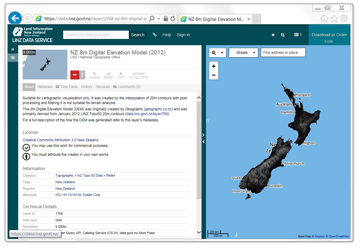
You could download the entire elevation data set as a single 31 GB file, but you’d be waiting quite a while! So let’s zoom in to the Auckland area and select some extents that are cropped to our area of interest, including the locations of any tidal boundary conditions we may wish to apply. Be sure to note the applicable projection:

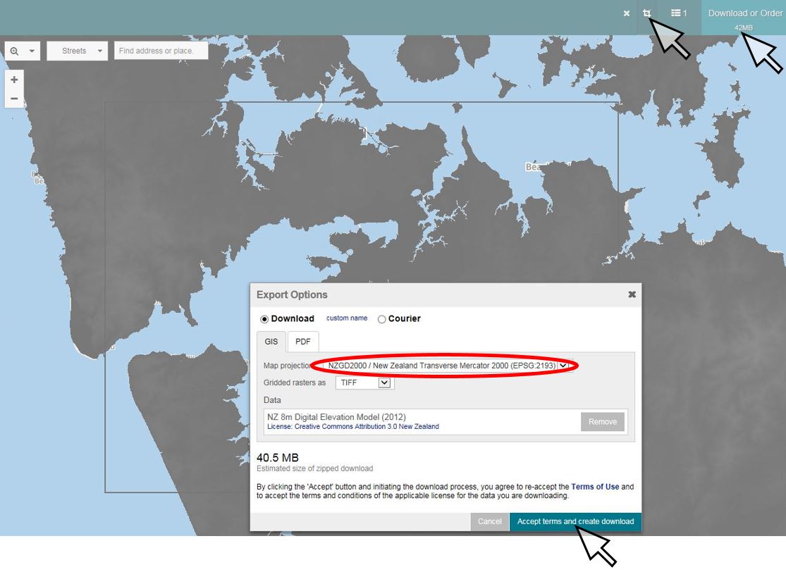
The cropped file is 40 MB in size, which is much more manageable than 31 GB! Keep in mind, though, that this data is derived from a much coarser data set, so it doesn’t really give us the stated 8-metre by 8-metre resolution accuracy, but it should be sufficient for our purposes here.

[A 1-metre DEM is also available for free download over this area, but even when cropped the file sizes for that data set are a bit too large for tutorial purposes.]

Now we need a projection file corresponding to the assigned projection of the downloaded DEM, which we noted from the LINZ server as NZGD2000. Just Google “NZGD 2000” and it should take you to spatialreference.org where you can download the .prj file. Here’s a screen shot of the website:

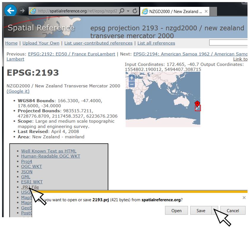Click on the link labelled “.PRJ File” and save the file to the project folder.

[I like to keep my projection files in a projection folder within a GIS subdirectory. If you’re following along with this exercise, you may wish to create those folders now, along with separate folders for terrain, aerial imagery, hydrology, and any other data categories you might need. I also always recommend renaming the projection file to “NZGD2000 NZTM Projection.prj” or something similarly descriptive. That way you can always link RAS Mapper to the same file rather than just choosing a random projection file that’s associated with one of your shape files. This avoids the risk of grabbing a shape file that’s in a different projection and also avoids confusion with HEC-RAS project .prj files.]

Step 3: Add geospatial data to RAS Mapper

We won’t cover these steps in detail here, since they’re covered in our Workshop #1, which is available for download here with screen shots of each step. In short, we’ll do the following:

Open HEC-RAS
Click on use “File | New Project” to start a new HEC-RAS project in SI units
Open RAS Mapper
Set the projection using “Tools | Set Projection” and browse to the NZGD 2000 prj file
Create a new terrain using “Tools | New Terrain” and browse to the downloaded DEM file (use the drop-down button to show “all file types” if you downloaded the DEM in asc format).
Add web imagery and assign transparency to confirm that we are projected to the right location
Add any other available shape files or static aerial imagery

If you turn everything off except the terrain file, you should see something like this in RAS Mapper (I’ve manually added the canal location to this screen shot to show where we’ll be working):

If you haven’t done so previously, try playing around with cutting profiles, adjusting upper and lower display limits in the legend, adding contours, adjusting hill shading, etc. Keep in mind that the white areas shown have no terrain data; in other words, each of those pixels in the DEM has been assigned a -99999 or similar value that is recognised by RAS Mapper and other CAD/GIS applications as the absence of data.

Step 4: Add bathymetry to the terrain data

Because there is no bathymetry in this data set, any 2D computations that touch the “no data” zone would fall apart. We want this model to cover coastal regions, so we’ll need to add some terrain data to represent the sea bed. We could download bathymetric data and merge the terrains together, but for our purposes, we can just invent some bathymetry to add to our terrain. Here is a summary of the process I took:

Open the Geometric Data Editor
Create a new 1D river reach (even though we won’t be using it to apply any flow, keep in mind that for orientation purposes the reach will be assigned a “flow direction” that assumes you are delineating the reach from upstream to downstream)
Note the reach length (GIS Tools | Reach Invert Lines Table | Compute Line Length) [mine is 20,000 metres long]
Add a new cross section at the “downstream” extent of the delineated reach (Station 0)
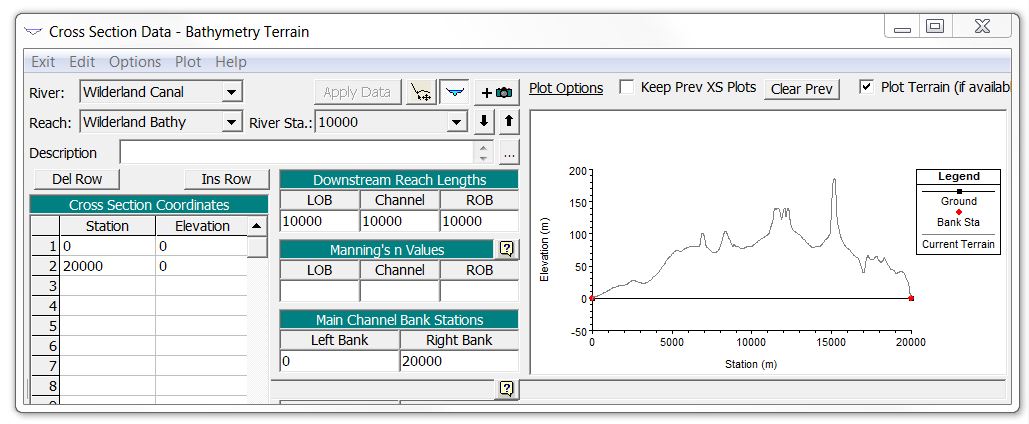
Enter cross section data for the downstream section (for this one I just made a two-point section with a beginning station of 0 and an end station equal to the reach length of 20,000 m, both with an elevation of -20 m)
Enter bank stations matching the end points of the cross section and enter downstream reach lengths of 0 for left, right, and channel
Copy the cross section to the middle of the reach by assigning a station ID equal to half the measured reach length (10000 for mine); use this same value as the downstream reach lengths in the cross section data
Copy the cross section to the “upstream” end of the reach by assigning a station ID equal to the measured reach length (20000 for mine), and use half the length (10,000 m) as the downstream reach lengths in your cross section (just leave it the same as the previous section)
Assign elevations to your sections (for this case I just kept the elevations at -20m elevation at the upstream and downstream ends, and changed them to 0m elevation for the middle section)
Save the geometry (if you tried to save it before adding features, you’ll lose your view extents – workaround here)

Here’s the middle cross section for reference:

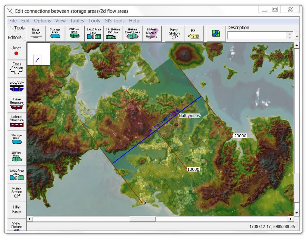
Here is the bathymetric geometry showing the extents of the 1D reach and cross sections. It’s just a rotated 20km by 20km square:

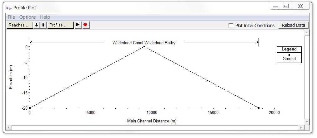
You can use the profile viewer in the main HEC-RAS window to check your elevations. Here is the profile view showing that the bathymetry is at an elevation of zero along our middle section and an elevation of -20m at the end sections:

This might seem like a tedious process, but once you’ve done a few of these, you’ll probably be able to set up similar geometries for terrain manipulation in just a couple of minutes. If you want to take it further, these steps are covered in more detail in some of the links listed in our terrain manipulation article.

This particular example doesn’t include much subsurface detail, but you can get as complex as you wish with the terrain modification option. In other examples, I’ve been able to get reasonably good definition out of the resulting terrain by aligning the cross section locations with the shoreline and estimated bathymetric contour lines. [Be sure to “accept displayed location as georeferenced” for each section if you’re going to do anything complicated.]

Step 5: Add the canal to the terrain data

Now let’s repeat the above steps to add the canal, using a new geometry (“File | New Geometry Data”).

[Keep in mind that both of these geometries are “orphans” that won’t be linked to any flow or plan files – their sole purpose is to manipulate terrain data.]

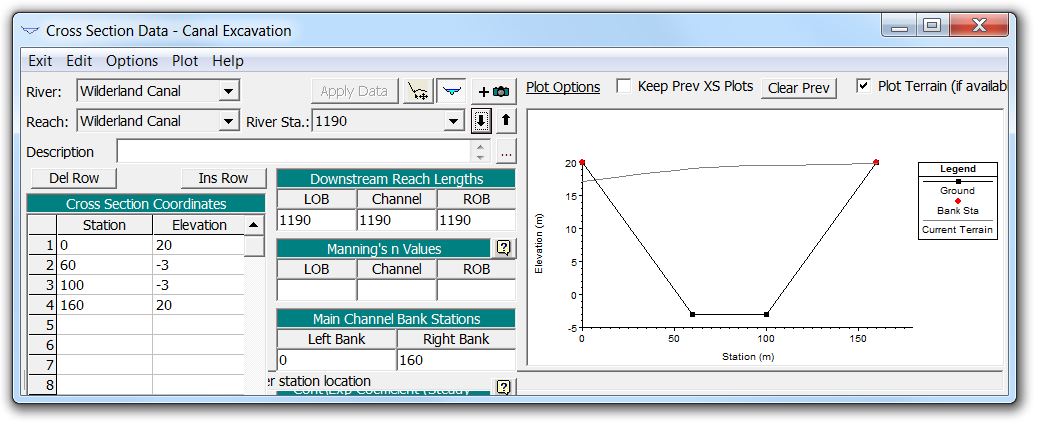
For this case, I’ve made a trapezoidal cross section at the upstream and downstream ends with a 40-metre bottom width and 2H:1V side slopes. I’ll assign a bottom elevation of -3 metres along the entire canal. The cross sections at the upstream and downstream end of the reach extend from the bottom elevation of -3 m to a top of bank elevation of +2 m. I’ve added a cross section in the middle that extends from -3 m up to +20 m to more closely match the daylight extents of the excavated slope. Here’s the middle cross section:

Here’s how the canal geometry looks with my 1D reach.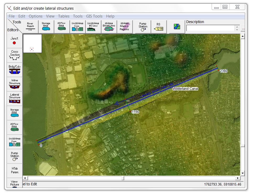

After saving this geometry, I’ll go straight to RAS Mapper for the next terrain manipulation steps (without saving any plan data). In RAS Mapper:

Right-click on the layer for the bathymetric geometry file
Select “Export Layer | Create Terrain Geotiff” (my bank stations cover the entire cross section extents, so it doesn’t matter whether I select “overbanks” or “channel only”)
Assign a name and resolution (I used a resolution of 8 metres to match the LINZ data) and click “Save” to create a geotif DEM of the reach with the 1D cross sections
Repeat the above steps for the canal, using a finer resolution that will capture the grade breaks, side slopes, and bottom width of the canal (I used 2 metres for mine)
Select “Tools | New Terrain”
Add each of the terrains using the Plus button
Stack the terrain files in order, with bathymetry at the bottom, the LINZ 8-metre DEM in the middle, and the canal at the top
Assign a name for the merged terrain hdf file and click “Create”
Zoom to the terrain and ensure that there are no white “no data” areas in the area you want to model

Step 6: Draw a 2D Flow Area

Next we’ll need to again create a new geometry file using the Geometric Data Editor, but this one will be linked to our flow and plan files.

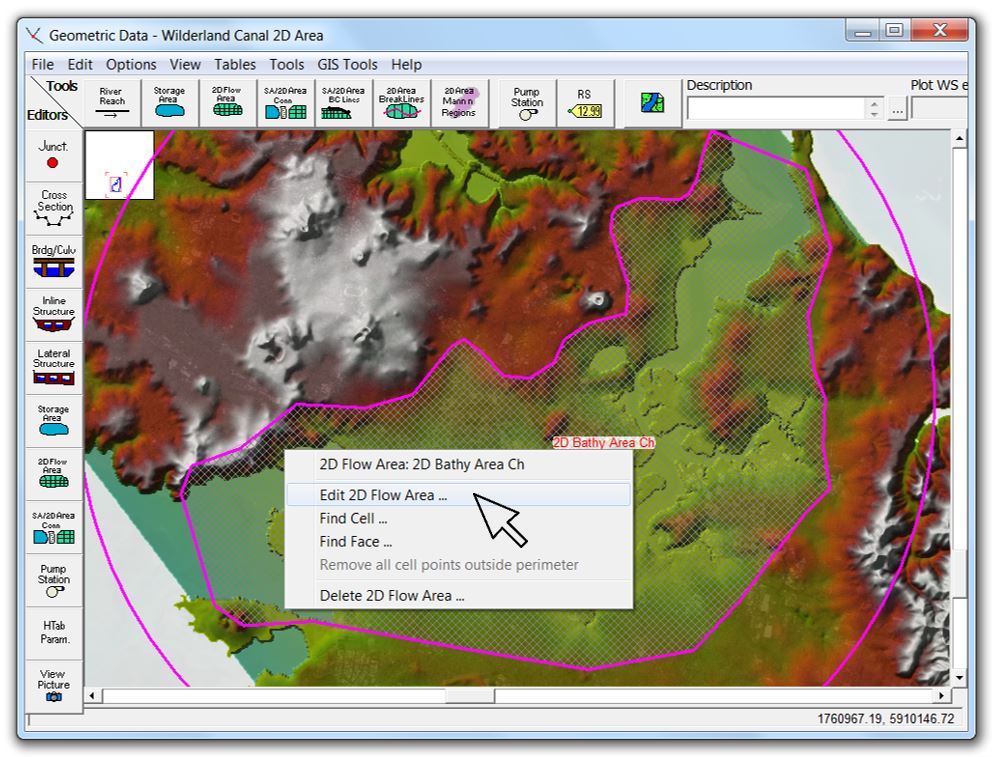
Click on the “2D Flow Area” icon in the Geometric Data Editor and delineate the extents of the model coverage. You may wish to roughly follow a colour band or contour line that exceeds any expected inundation levels. Be sure that you’re happy with the shape of the outer extents of your 2D area where it crosses the seafloor in particular, since the boundary condition lines for inflow and outflow will snap to the outer boundary.

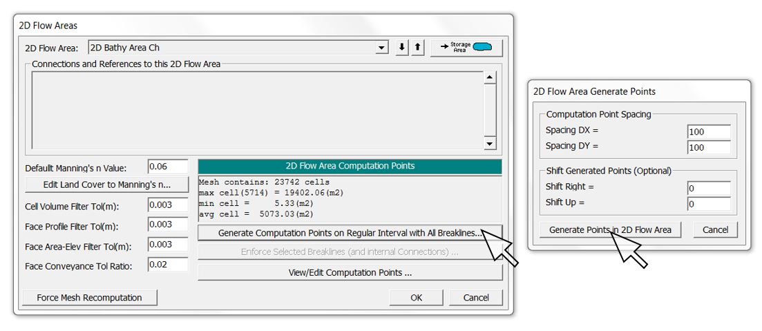
Select the 2D area and choose “Edit 2D Area”. Select the “Generate Computation Points” button and assign a mesh resolution (I’ll use a very coarse grid size of 100-metres by 100-metres as a first pass).

Save the geometry, then go back to RAS Mapper, right-click on the geometry, and associate the merged terrain file with the new geometry.

Step 7: Add boundary conditions and breaklines

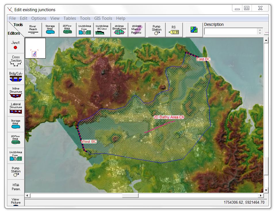
Next we’ll create boundary conditions along the eastern and western extents of the bay. Go back into the geometry editor and click on the SA/2D Area BC Lines button. Since these boundary conditions will be used with stage hydrographs (that will allow discharge to pass in both directions), the left-right positive flow orientation is a bit arbitrary. Draw the line clockwise along the 2D Flow Area if you want outflow to be positive, anticlockwise for positive inflow). I’ve called one of my boundaries “West BC” and the other “East BC” as shown here:

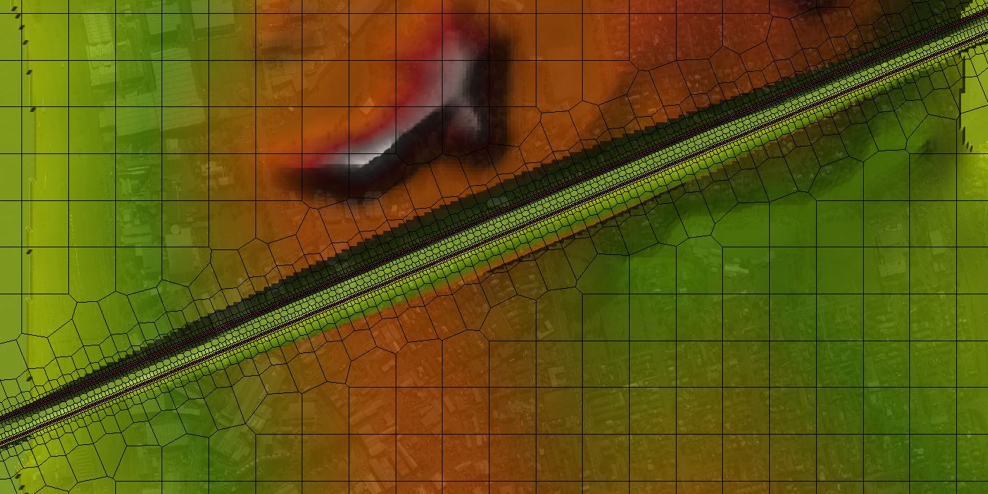
Next we’ll add breaklines along the canal alignment using the “2D Area Break Lines” button. I drew one along the left toe of slope and one along the right toe of slope. Click on each breakline and assign a minimum breakline cell spacing (I used 2 metres), and enforce the breaklines. Once you’ve enforced the breaklines, check the resulting cell shapes to make sure that cell faces are generally oriented parallel or perpendicular to the flow direction in the canal. Try to fix any “red dot” errors by adjusting minimum/maximum cell spacing values, or moving/adding breaklines.

[It’s probably good practice to fix errors with breaklines rather than adding/moving/removing individual computational points, since in the latter case you would have to redo the edits manually every time you recompute your overall mesh.]

Here’s how my cell alignment looks after enforcing my breaklines:

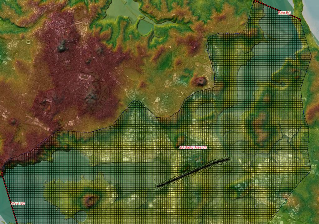
For this case, flow will stay confined within the canal; if we were looking at overtopping flows, we would also want breaklines along the crest at the top of slope. Here’s the overall layout of the geometry showing the 2D mesh, the boundary conditions and the breaklines:

Save the geometry file and the project file as well just to be safe.

Step 8. Enter stage hydrographs in the unsteady flow file

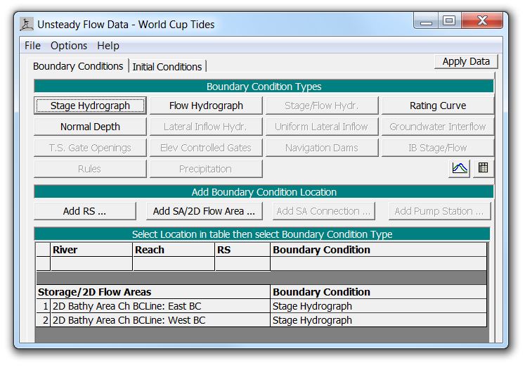
Open the unsteady flow data editor and save the file with a title indicating the time series you’ll be using for the simulation. I’ve called mine “World Cup Tides” (sorry – spoiler for those who haven’t yet guessed the significance of Halloween 2015!)

Click on the blank cells under the Boundary Condition column at the bottom of the window and select “Stage Hydrograph.”

[Keep in mind that using “Stage Hydrograph” as a boundary condition carries with it the assumption that the water body on the opposite side of the boundary condition is an infinitely large storage area and that the flow volumes crossing the boundary are insignificant by comparison and do not affect the stage-volume relationship of the external water body. That’s certainly the case with the ocean, but it may not necessarily be the case in the locations within the bays where I’ve drawn my boundary conditions.]

Next, highlight each boundary condition and click on the “Stage Hydrograph” button to enter the time series.

We could break the tidal curves down with as much detail as we wish (trying to make ideal sine curves out of the peaks and troughs with minute-by-minute values, for instance.) For simplicity here, I’ll use a 30-minute time interval and just enter the four recorded values (HW, HHW, LW and LLW) in the closest corresponding increment. Click on “Interpolate Missing Values” to populate the blank cells as shown here:

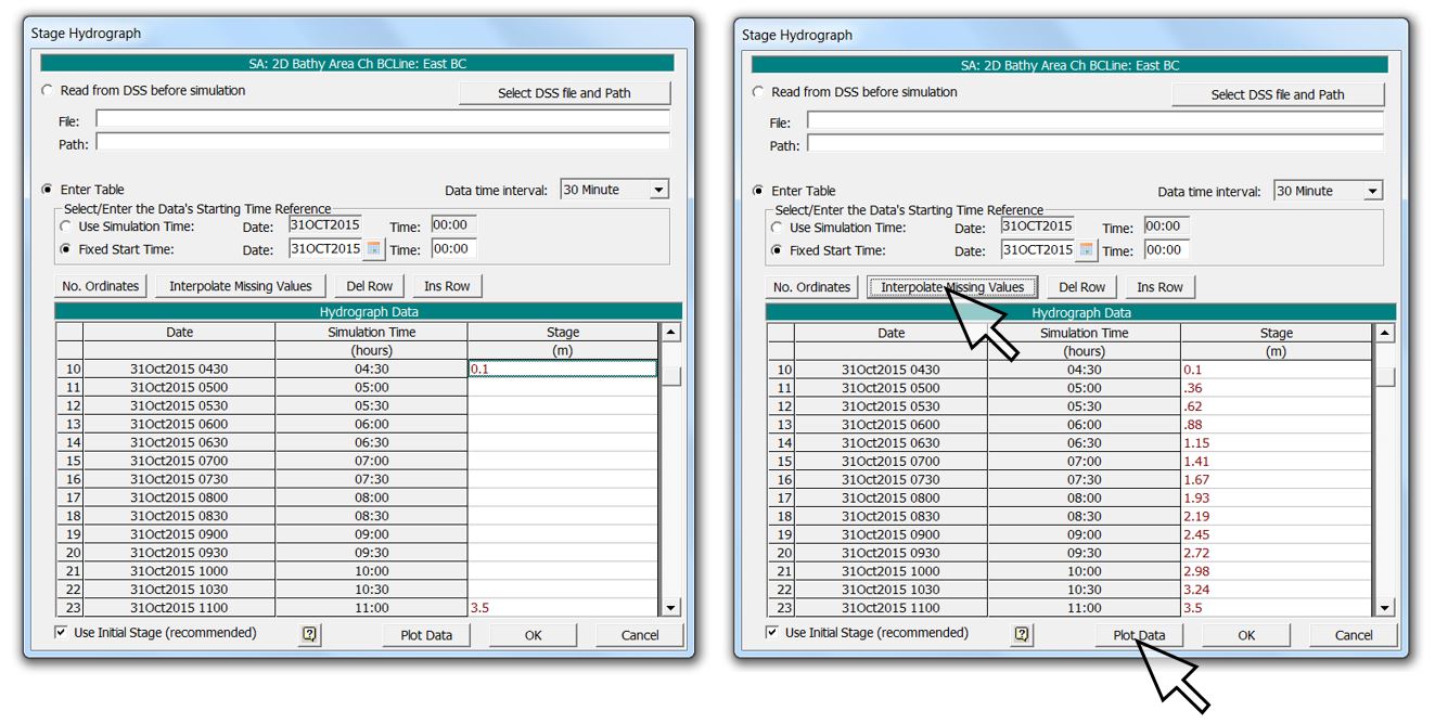
[By the way, the interpolate feature makes for a nice little trick when you have a table in Excel or other spreadsheet with variably spaced data that you want to interpolate. Sometimes I’ll take a column in a file that has nothing to do with hydraulics and paste it into the unsteady flow hydrograph table in HEC-RAS just to interpolate the values and then paste the column back to my spreadsheet.]

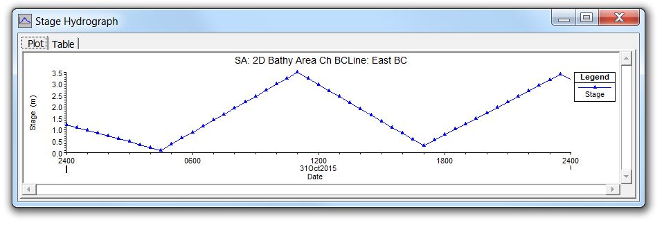
It’s always a good idea to click the “Plot Data” button to check the graphical chart for any typos in the tabulated data. Here’s how the East BC series looks:

To compare the phasing, I clicked on the Table tab and copied the values for both hydrographs into Excel: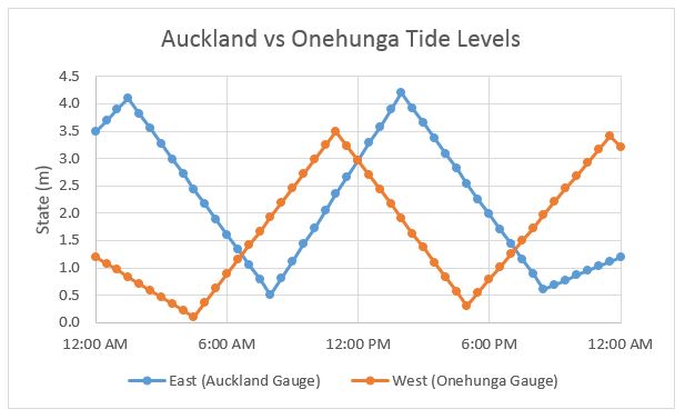

The chart shows that the peaks are out of phase by about three hours.

[Keep in mind that the higher of the two starting stages assigned to the first time step will by default become the initial condition water surface elevation across the entire 2D Flow Area. The initial levels could be adjusted in a number of ways, such as using separate 2D Flow Areas for the two bays and the canal that are connected with a SA/2D Area Connection. The canal itself could in fact be modelled as a 1D reach that is coupled with the 2D areas; instabilities tend to arise at the interfaces, though, and given the troubleshooting time involved, personally I find it much easier to keep it all in 2D!]

Save the flow file before moving on.

Step 9. Set up and run the unsteady plan file

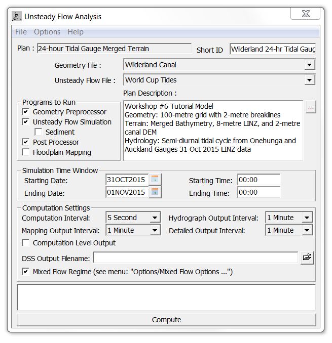
Open the Unsteady Flow Analysis window and save with a title that indicates which geometry and flow files are being combined. I always recommend including a detailed description of the run in the Plan Description window as well. Set the simulation window to match the 24-hour period corresponding to the tidal data.

Use your minimum grid size and assumed maximum velocities (with wave celerity, if significant) to estimate a computational time step based on Courant Number criteria (Search for “Courant Number” in the 2D Manual if you need a reference for the equation and guidelines). Set the other intervals as desired, making sure that they will give you enough frames to make a smooth animation and enough data points to adequately interpret the results. Here are the values I’m using for my initial run:

Any model with significant wetting and drying (which includes pretty much every coastal model) should be run with the Full Momentum equation set rather than the default Diffusion Wave simplification (selected from the Unsteady Flow Analysis window under “Options | Calculation Options and Tolerances | 2D Flow Options | Equation Set”). In this case the selected equation set doesn’t make a huge difference in water surface levels, but the velocity vectors will differ quite significantly between the two methods. If you choose to apply the Diffusion Wave method – generally to save computation time – it’s usually worth running at least one sensitivity analysis to check the impact on your results. There may be a case for adjusting some of the other variables as well, but for this model, I’ve left all other parameters at their the default value.

Save the plan file and project and press “Compute” to run the plan. This is the moment of truth for your model – hopefully you get through it error free! Otherwise it’s time for troubleshooting, which we won’t cover here, except to say that some errors can only be fixed by saving, closing, and re-opening HEC-RAS. If the error isn’t obvious, that trick might be your lowest hanging fruit on the troubleshooting tree.

Step 10. View and animate the results in RAS Mapper

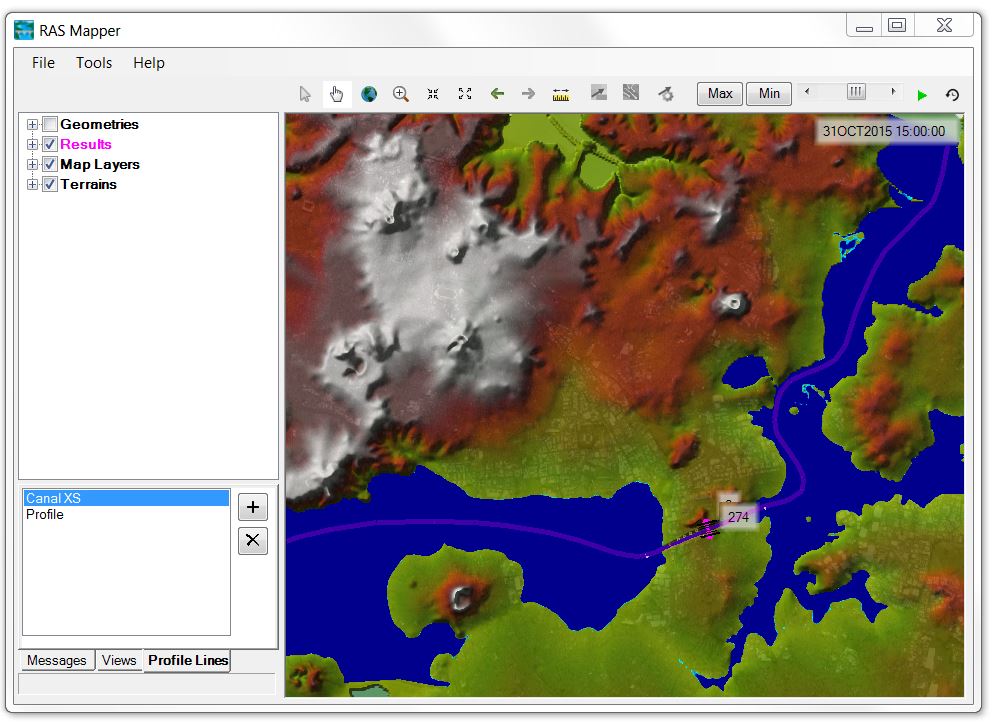
Now for the fun part: animating the results. Open RAS Mapper (re-open if it was still open from before the plan was run). Click on the “Profile Lines” tab and add a long section profile through the canal and another one crossing the canal as a cross section:

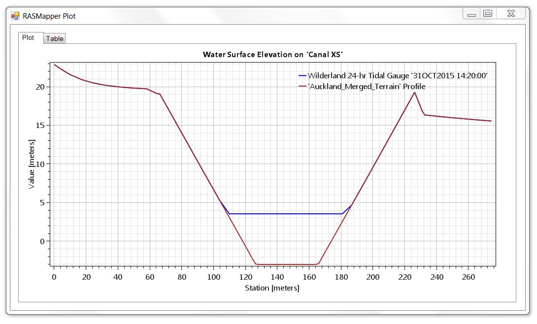
Right-click on the “Canal XS” profile and plot the WSE and the time series flow data. Here is the cross section showing the terrain along with the water surface elevation for the selected time step:

Here is the 24-hour hydrograph showing the reversing flux through the cross section:

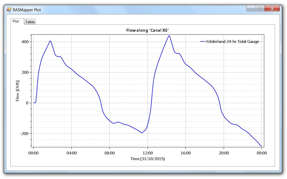
The cross section was delineated from north to south, so the positive flow direction is to the east (left-to-right looking downstream). Negative flows in the above hydrograph indicate flow to the west.

Next let’s have a look at the long section view through the canal. Right-click on the profile to view the WSE plot as shown here for a selected time step:

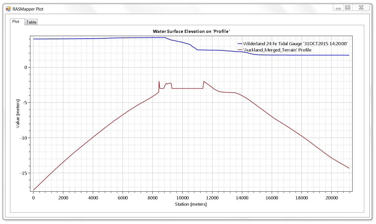
This profile shows a differential head of approximately 2.5 metres between the east and west ends of the canal. This is for a single time step, but the slider bar can be used to animate the plan and profile view together. Here is an animation showing both the plan and profile view together:

We can also generate plots for velocity, shear, D*V, stream power or a number of other variables that you may wish to observe. Here is a velocity map for a single selected time step:

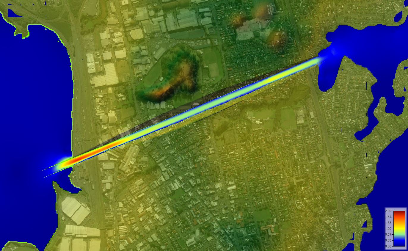
[Keep in mind that in a model with lots of flow reversals, “Max” plots can look a bit strange, since two adjacent pixels might be displaying values that occurred hours apart and in completely opposite directions.]

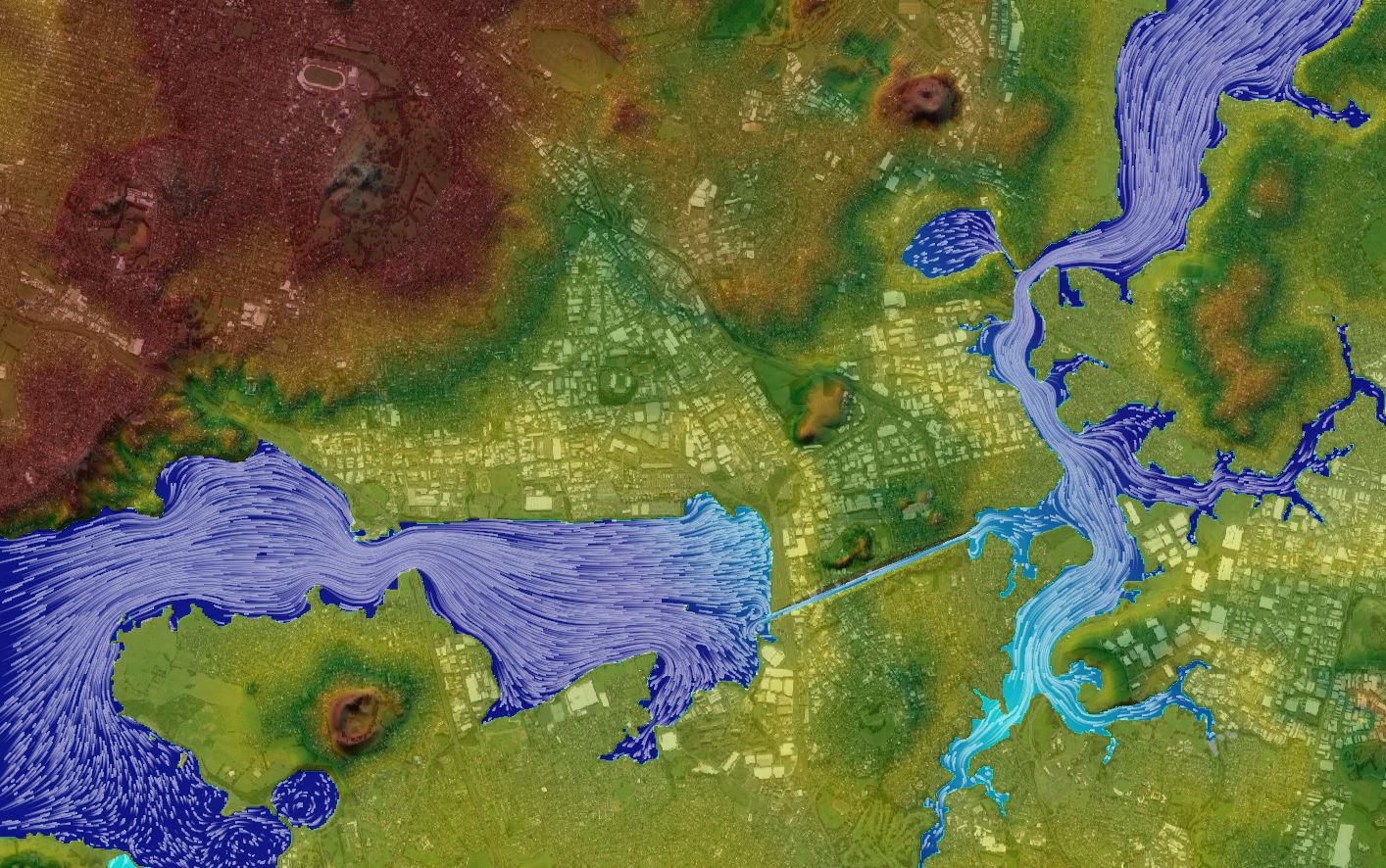
Try turning on particle tracing to watch the flow patterns at any given time step. [Keep in mind that particle tracing does not relate to any actual travel time for the paths shown, but is rather just an animation of the relative velocity vectors taken at the cell face points at that particular instantaneous time step.]

You can adjust the speed and density in the settings to fine-tune the appearance:

Here’s a zoomed in version showing the western inlet:

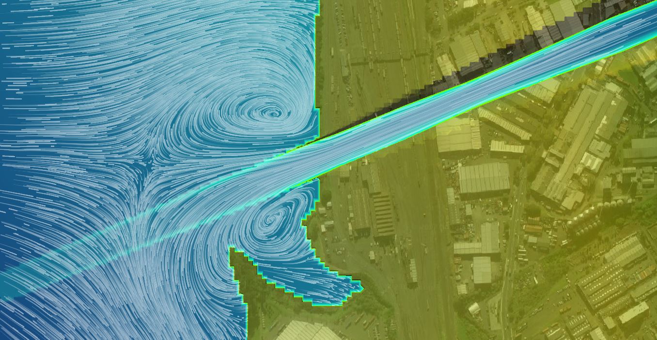
The accuracy of the circulation patterns won’t be all that great, especially since we made up the bathymetry and we’re using 100-metre computational grids, but you can still see some cool eddy patterns, provided you have run your model using the Full Momentum equation set rather than the default Diffusion Wave simplification. If you want to try an interesting sensitivity, try saving the plan file under another name and run it again as Diffusion Wave. Although the water surface levels will be almost identical between the two equation sets, the circulation patterns exhibited by the particle tracing will be wildly different!

By the way, if you want to record an animation of the particle tracing or a dynamic inundation map in RAS Mapper, you’ll need to use third-party screen capture software, since unfortunately there’s no built-in recording capability in HEC-RAS. If you have PowerPoint, you can simply choose “Insert | Screen Recording” from the main menu and drop the video into a presentation:

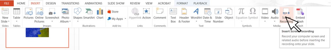
If you right-click on the video in PowerPoint, you can save the media file to your hard drive, which is what I’ve done with the clips below. Video files can get very large, so I like to pull in short clips maybe 5 seconds or so in length showing the particle tracing, and then just set them on repeat. That way it looks like a continuous animation while you have a PowerPoint slide up on the screen – with a very small file size. Here is a clip showing the whole canal and another one other zoomed to the inlet; these are taken at different time steps with the flow having reversed in the meantime:

Next Steps

Well, we’ve reached the end of the road for this tutorial, but this would really just be the beginning if we were doing a real model for a proposed design. With our initial run complete, this is where the iterations would begin. Now would be the time to go back and look at the results – flow directions, velocities, inundation levels, etc. – to see where we should refine cell spacing, breaklines, time steps, roughness values, etc., or make any number of other refinements.

If we could trust these model results – which, after all, have come from a model that we can build from scratch in an introductory course in less than an hour – consultants could get by with charging a hundred dollars for a model, and you’d be on your way. So why do bona fide models cost thousands or even hundreds of thousands of dollars? Well these results may look cool, but unfortunately they’re entirely bogus!

Of course we would need real bathymetry for this one to be meaningful in any way, but we would also want to do some further sensitivity testing, without which no model is complete. At a bare minimum, a roughness sensitivity is usually needed, since roughness values are just estimates with quite a bit of uncertainty. A roughness sensitivity allows results to be presented as a range rather than absolute values, or – if presented as single values – accompanied by confidence limits. In addition, a time step sensitivity analysis is also a good idea in order to confirm that your results converge.

In this case there’s obviously no available calibration data, but for models that do have calibration data available, various parameters can be tweaked after the initial run in order to match measured flow or stage data. If this were a real project, we may want to recommend installing additional gauges to monitor tidal levels near the boundary conditions and proposed canal inlet locations, with observations correlated to historical measurements at existing gauges.

While it makes an interesting case study, HEC-RAS is probably not the optimal software for this particular application. To really get this one right, you might make the case for a full 3D hydrodynamic coastal model that accounts for vertical mixing, currents, wave runup, wind setup, etc. In that case, HEC-RAS might be used for the canal reach and coupled with a coastal model that assigns HEC-RAS boundary conditions where the canal hits the bays.

Despite the limitations, the approach we’ve taken with this preliminary HEC-RAS model can give us a good start in figuring out what to do next. Refinements would be made using the same steps that we’ve covered here, so hopefully the exercise was useful in getting up and running with terrain manipulation and tidal boundary condition.

Please feel free to contact me with any suggestions for improving this article or if you need any help setting up your own models.

Krey Price
Surface Water Solutions

* 31 October 2015: The All Blacks defeat Australia to become the first team in history to repeat as Rugby World Cup champions!